4 Gradually varied flow

4.1 Channel Slope and Friction

In the previous section of rapidly varied flow little mention was made of losses due to friction or the influence of the bed slope. It was assumed that frictional losses were insignificant - this is reasonable because rapidly varied flow occurs over a very short distance. However when it comes to long distances they become very important, and as gradually varied flow occurs over long distances we will consider friction losses here.

In the section on specific energy, 3.2, it was noted that there are two depths possible in uniform flow for a given discharge at any point in the channel. (One is super-critical the other sub-critical.) The solution of the Manning equation results in only one depth - the normal depth.

It is the inclusion of the channel slope and friction that allows us to decide which of the two depths is correct. i.e. the channel slope and friction determine whether the uniform flow in the channel is sub or super-critical.

The procedure is

1.

Calculate the normal depth from Manning’s equation 2.13
2.

Calculate the critical depth from equation 3.20

The normal depth may be greater, less than or equal to the critical depth. Comparing these enables us to identify whether we have sub or super-critical flow in the channel:

•

if the normal depth greater than critical depth then flow is sub-critical
•

if the normal depth less than critical depth then flow is super-critical

An alternative way to view this is to examine the channel slope for a given roughness.

For a given channel and roughness there is only one slope that will give the normal depth equal to the critical depth. This slope is known as the critical slope ( $S_{c}$ ).

If the slope is less than $S_{c}$ the normal depth will be greater than critical depth and the flow will be sub-critical flow. The slope is termed mild.

If the slope is greater than $S_{c}$ the normal depth will be less than critical depth and the flow will be super-critical flow. The slope is termed steep .

4.1.1 Transitions between sub and super-critical flow

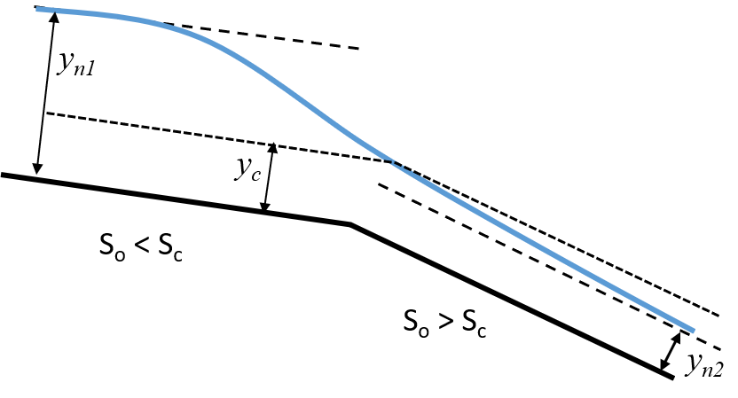
If sub-critical flow exists in a channel of a mild slope and this channel meets with a steep channel in which the normal depth is super-critical there must be some change of surface level between the two. In this situation, the surface changes gradually between the two. The flow in the joining region is known as gradually varied flow), (GVF).

This situation can be clearly seen in the figure on the left below. Note how at the point of joining of the two channels the depth passes through the critical depth.

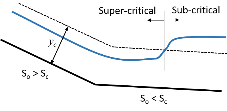
Refer to caption — (a) Sub-critical to Super-critical

If the situation is reversed and the upstream slope is steep, super-critical flow, and the downstream mild, sub-critical, then there must occur a hydraulic jump to join the two. There may occur a short length of gradually varied flow between the channel junction and the jump. The figure above right shows this situation:

Analysis of gradually varied flow can identify the type of profile for the transition as well as position hydraulic jumps.

4.2 The equations of gradually varied flow

The basic assumption in the derivation of this equation is the assumption that the change in energy with distance is equal to the friction loses.

\frac{dH}{dx}=-S_{f}

(4.1)

Taking the Bernoulli equation, eqn: 3.7, (repeated here):

y+\frac{\alpha V^{2}}{2g}+z=H

(4.2)

and differentiating and equating to the friction slope

\frac{d}{dx}\left(y+\frac{\alpha V^{2}}{2g}\right)=-\frac{dz}{dx}-S_{f}

(4.3)

or using the bed slope definition

S_{o}\left(=-\frac{dz}{dx}\right)

(4.4)

\frac{dE_{s}}{dx}=S_{o}-S_{f}

(4.5)

We saw earlier how specific energy changes with depth (derivation of Equation 3.20)

\frac{dE_{s}}{dx}=1-\frac{Q^{2}B}{gA^{3}}=1-F_{r}^{2}

(4.6)

Combining this with equation 4.5 gives

\frac{dy}{dx}=\frac{S_{o}-S_{f}}{1-F_{r}^{2}}

(4.7)

This is the basic equation of gradually varied flow. It described how the depth, $y$ , changes with distance $x$ , in terms of the bed slope $S_{o}$ , friction $S_{f}$ and the discharge, $Q$ , and channels shape (encompassed in $F_{r}$ ).

Equations 4.5 and 4.7 are differential equations equating relating depth to distance. There is no explicit solution (except for a few special cases in prismatic channels). Numerical integration is the only practical method of solution. This is normally done on computers, however it is not too cumbersome to be done by hand.

4.2.1 Friction slope, $S_{f}$ , in gradually varied flow

For the determination of the friction slope in gradually varied flow we make the assumption that energy loss is the as in uniforn flow. Recall that in uniform flow the friction slope is equal to the bed slope i.e. $S_{o}=S_{f}$ .

In uniform flow, we have the Chezy (2.7) or Manning’s (2.11) equations, which written in terms of $V$ with the friction slope equated to the bed slope are:

V=C\sqrt{RS_{f}}

and

V=\frac{1}{n}R^{2/3}S_{f}^{1/2}

Rearranging these gives expressions we can use for $S_{f}$ in gradually varied flow:

S_{f}=\frac{V^{2}}{C^{2}R}

(4.8)

S_{f}=\frac{n^{2}V^{2}}{R^{4/3}}

(4.9)

or, in terms of $Q$

S_{f}=\frac{n^{2}Q^{2}}{R^{4/3}A^{2}}

(4.10)

4.2.2 Critical Slope, $S_{c}$ , evaluation

We have the Manning’s equation 2.13 that gives normal depth

Q=\frac{1}{n}\frac{A^{5/3}}{P^{2/3}}S_{o}^{1/2}

and equation 3.20 for $F_{r}$ at critical depth (taking $\alpha=1$ )

\frac{Q^{2}B_{c}}{gA_{c}^{3}}=1

Rearranging these in terms of Q and equating gives:

\frac{1}{n}{}\frac{A_{c}^{5/3}}{P_{c}^{2/3}}S_{c}^{1/2}=\sqrt{\frac{gA_{c}^{3}% }{B_{c}}}

(4.11)

S_{c}=\frac{gn^{2}P_{c}}{B_{c}R_{c}^{1/3}}

(4.12)

(Note that the $c$ subscript indicates that these parameters are all at critical depth.)

Critical Slope for a Wide Channel

For the simple case of a wide rectangular channel, width $B=b$ , $A=by$ and $P\approx b$ , then the above equation becomes

S_{c}=\frac{gn^{2}}{y_{c}^{1/3}}

(4.13)

Note that this equation is explicit in either $S_{c}$ or $y_{c}$ , so either are straightforward to calculate.

4.3 Classification of profiles

Before attempting to solve the gradually varied flow equation a great deal of insight into the type of solutions and profiles possible can be gained by taking some time to examine the equation. Time spent over this is almost compulsory if you are to understand steady flow in open channels.

For a given discharge, $S_{f}$ and $F_{r}^{2}$ are functions of depth.

S_{f}=\frac{n^{2}Q^{2}}{R^{4/3}A^{2}}

(4.14)

F_{r}^{2}=\frac{Q^{2}B}{gA^{3}}

(4.15)

A quick examination of these two expressions shows that they both increase with $A$ , i.e. increase with $y$ .

We also know that when we have uniform flow

S_{f}=S_{o}\qquad\text{and}\qquad y=y_{n}

S_{f}>S_{o}\qquad\text{when}\qquad y<y_{n}

S_{f}<S_{o}\qquad\text{when}\qquad y>y_{n}

and

F_{r}^{2}>1\qquad\text{when}\qquad y<y_{c}

F_{r}^{2}<1\qquad\text{when}\qquad y>y_{c}

From these inequalities, we can see how the sign of $dy/dx$ i.e. the surface slope changes for different slopes and Froude numbers.

Taking the example of a mild slope, shown in the figure 2(a) below:

The normal and critical depths are shown (as it is mild, normal depth is greater than critical depth). Treating the flow as to be in three regions:

•

region 1, above the normal depth. Here will be $M1$ surface profile.
•

region 2, between normal and critical depth. Here will be $M2$ surface profile.
•

region 3, below critical depth. Here will be $M3$ surface profile.

The direction of the surface inclination may thus be determined for each region. Remembering equation 4.7

\frac{dy}{dx}=\frac{S_{o}-S_{f}}{1-F_{r}^{2}}

region 1

y>y_{n}>y_{c}\qquad Sf<So\qquad F_{r}^{2}<1\qquad\Rightarrow\qquad dy/dx\text{% is positive, surface rising}

region 2

y_{n}>y>y_{c}\qquad S_{f}>S_{o}\qquad F_{r}^{2}<1\qquad\Rightarrow\qquad dy/dx% \text{ is negative, surface falling}

region 3

y_{n}>y_{c}>y\qquad S_{f}>S_{o}\qquad F_{r}^{2}>1\qquad\Rightarrow\qquad dy/dx% \text{ is positive,surface rising }

The condition at the boundary of the gradually varied flow may also be determined in a similar manner:

region 1

\text{As }y\rightarrow\infty\text{ then }S_{f}\text{ and }F_{r}\rightarrow 0% \text{ and }dy/dx\rightarrow S_{o}

Hence the water surface is asymptotic to a horizontal line for it maximum

\text{As }y\rightarrow y_{n}\text{ then }S_{f}\rightarrow S_{o}\text{ and }dy/% dx\rightarrow 0

Hence the water surface is asymptotic to the line $y=y_{n}$

region 2 As for region 1 as $y$ approaches normal depth:

\text{As }y\rightarrow y_{n}\text{ then }S_{f}\rightarrow S_{o}\text{ and }dy/% dx\rightarrow 0

Hence the water surface is asymptotic to the line $y=y_{n}$

But a problem occurs when $y$ approaches the critical depth:

\text{As }y\rightarrow y_{c}\text{ then }F_{r}\rightarrow 1\text{ and }dy/dx\rightarrow\infty

This is physically impossible but may be explained by the pointing out that in this region the gradually varied flow equation is not applicable because at this point the fluid is in the rapidly varied flow regime. In reality a very steep surface will occur (and possibly a hydraulic jump).

region 3 As for region 2 a problem occurs when $y$ approaches the critical depth:

\text{As }y\rightarrow y_{c}\text{ then }F_{r}\rightarrow 1\text{ and }dy/dx\rightarrow\infty

Again we have the same physical impossibility with the same explanation. And again in reality a very steep surface will occur.

\text{As }y\rightarrow 0\text{ then }dy/dx\rightarrow S_{o}\text{ the slope of% bed of the channel}

The gradually varied flow equation is not valid here but it is clear what occurs (the channel is dry!).

In general (and key to remember),

•

normal depth is approached asymptotically
•

critical depth at right angles

The possible surface profiles within each region can be drawn from the above considerations. These are shown for the mild sloped channel below.

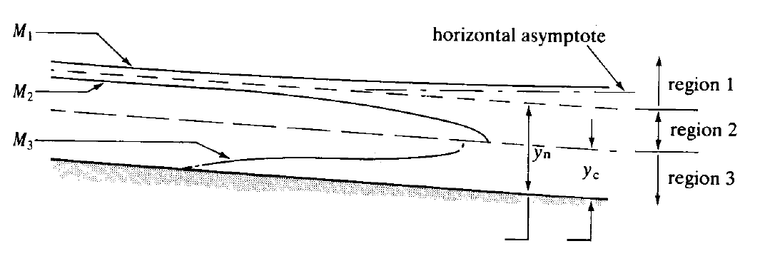
The surface profile in region 1 of a mild slope is called an M1 curve, in region 2 an M2 curve and in region 3 an M3 curve.

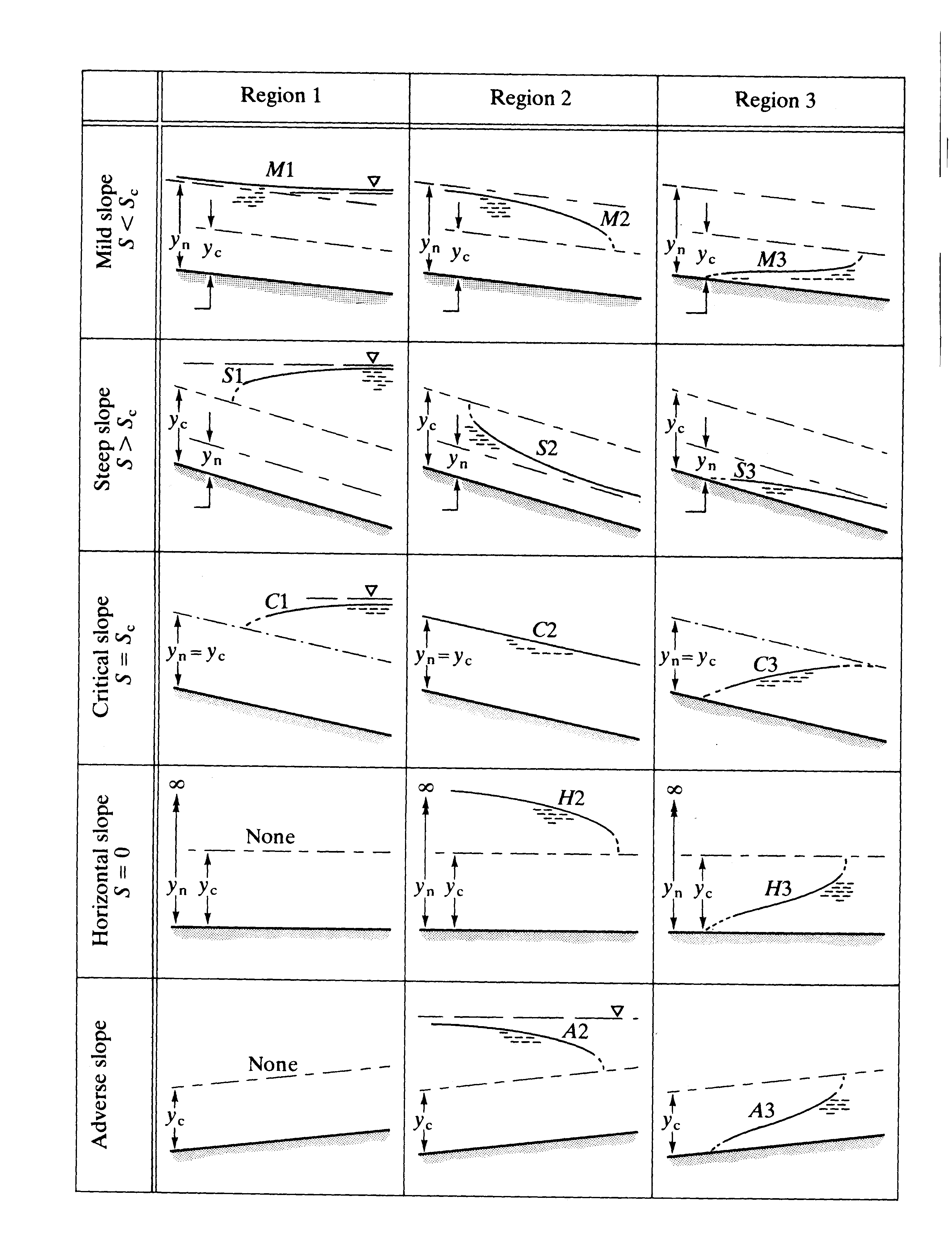
All the possible surface profiles for all possible slopes of channels (there are 15 possibilities) are shown in the figure 4.4 on the next page.

4.4 How to determine the surface profiles

Before one of the profiles discussed above can be decided upon two things must be determined for the channel and flow:

a

Whether the slope is mild, critical or steep. The normal and critical depths must be calculated for the design discharge
b

The positions of any control points must be established. Control points are points of known depth or relationships between depth and discharge. Examples are weirs, flumes, gates or points where it is known critical flow occurs like at free outfalls, or that the flow is normal depth at some far distance downstream.

Once these control points and depth positions have been established the surface profiles can be drawn to join the control points with the insertion of hydraulic jumps where it is necessary to join sub and super-critical flows that don’t meet at a critical depth.

Below are two examples.

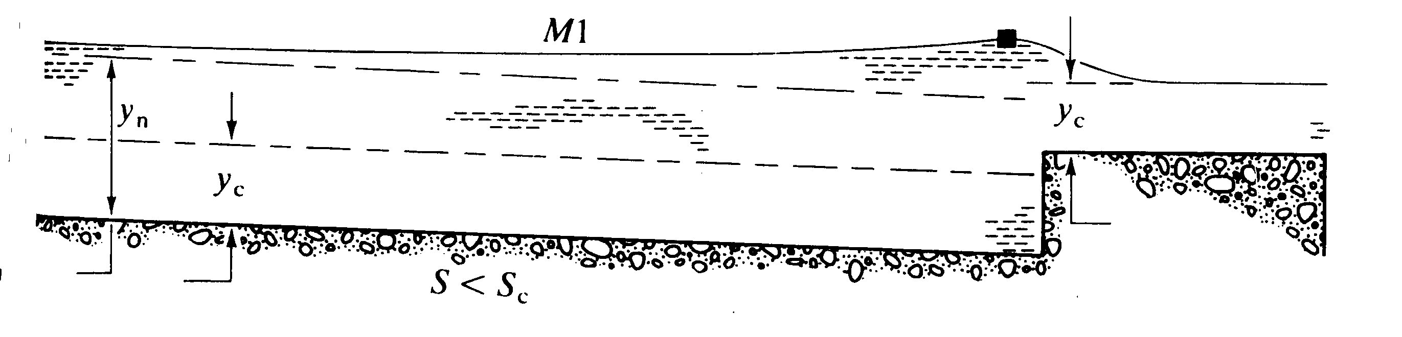
This shows the control point just upstream of a broad crested weir in a channel of mild slope. The resulting curve is an M1.

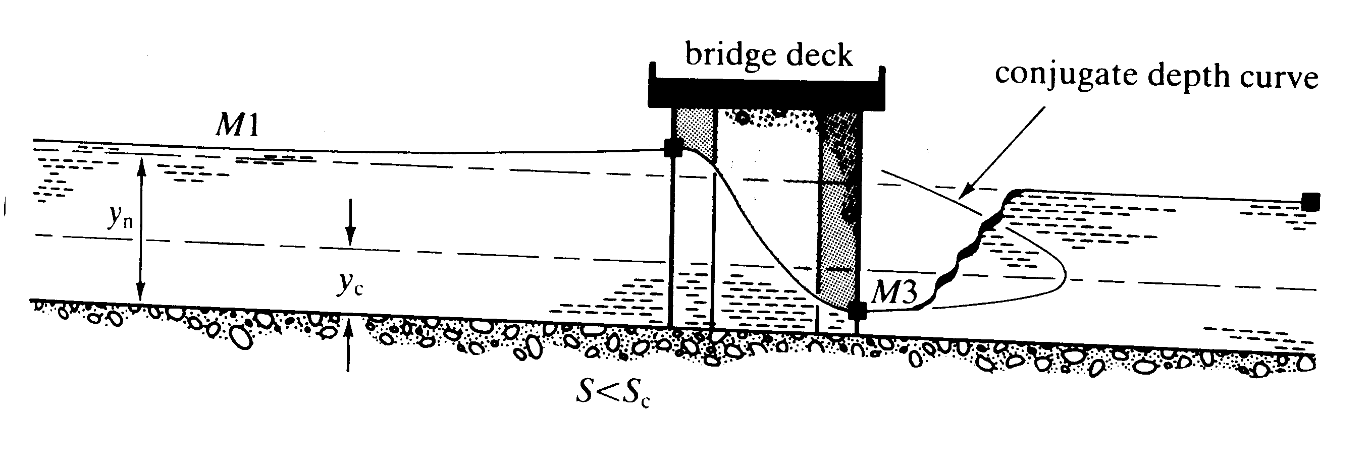
This shows how a bridge may act as a control - particularly under flood conditions. Upstream there is an M1 curve then flow through the bridge is rapidly varied and the depth drops below critical depth so on exit is super-critical so a short M3 curve occurs before a hydraulic jump takes the depth back to a sub-critical level.

4.5 Method of solution of the Gradually varied flow equation

There are three (equivalent) forms of the equations for gradually varied flow: Eqs 4.1, 4.5 and 4.7, which are respectively:

\frac{dH}{dx}=-S_{f}

\frac{dE_{s}}{dx}=S_{o}-S_{f}

\frac{dy}{dx}=\frac{S_{o}-S_{f}}{1-F_{r}^{2}}

In the past, direct and graphical integration methods have been used to solve the backwater equations, however, these methods have been superseded by numerical methods which should now be the only methods used.

4.5.1 Numerical methods

All (15) of the gradually varied flow profiles shown above may be quickly solved by simple numerical techniques. One computer program (or spreadsheet) can be written to solve most situations.

Historically these equations were solved by one of two numerical integration methods specifically designed for the gradually varied flow equation and to be done by hand, on paper. These are called:

i

Direct step - distance from depth
ii

Standard step method - depth from distance

While it is is perfectly fine to use these, and it is common to implement them in a program or a spreadsheet, it is probably now better to consider numerical methods developed for solving general ODEs (ordinary differential equation) which are formally defined in their accuracy (order) and implemented in many packages. Here they will be refereed to as a third method and named:

iii

Numerical Integration (e.g. Euler or Runge Kutta methods) - which can give either distance from depth or depth from distance and are of a quantifiable accuracy.
Further details of these are given in sections below.

Whichever method we use we will need to calculate $S_{f}$ , see section 4.2.1, that is calculated from the uniform flow equations to give, from Chezy eqn 4.8 or from Manning’s equation 4.10), i.e.:

S_{f}=S_{o}=\left(\frac{Q}{ACR^{1/2}}\right)^{2}=\left(\frac{Qn}{AR^{2/3}}% \right)^{2}

(4.16)

It is common to do this integration for examples of wide channels and use flow per unit width, $q$ . For this the equivalent formula is:

S_{f}=\left(\frac{qn}{y^{5/3}}\right)^{2}

(4.17)

4.5.2 The direct step method - distance from depth

This method will calculate (by integrating the gradually varied flow equation) a distance for a given change in surface height.

The equation used is eqn. 4.7, which written in finite difference form is

\Delta x=\Delta y\left(\frac{1-F_{r}^{2}}{S_{o}-S_{f}}\right)_{\text{mean}}

(4.18)

The steps in the solution are:

1.

Determine the control depth as the starting point
2.

Decide on the expected curve and depth change if possible
3.

Choose a suitable depth step $\Delta y$
4.

Calculate the term in brackets at the mean depth between the current (initial) depth and depth at the next step (i.e. $y_{\text{mean}}=y_{\text{initial}}+\Delta y/2$ )
5.

Calculate $\Delta x$
6.

Repeat 4 and 5 until the appropriate distance/depth change has been reached

This is really best seen demonstrated in an example.

4.5.3 The standard step method - depth from distance

This method will calculate (by integrating the gradually varied flow equation) a depth at a given distance up or downstream.

The equation used is 4.5, which written in finite difference form is

\Delta E_{s}=\Delta x(S_{o}-S_{f})_{\text{mean}}

(4.19)

The steps in solution are similar to the direct step method shown above but for each $\Delta x$ there is the following iterative procedure:

1.

Assume a value of depth $y$ (the control depth or the last solution depth)
2.

Calculate the specific energy $E_{s_{x}}$
3.

Calculate $S_{f}$
4.

Calculate $\Delta E_{s}$ using equation 4.19
5.

Calculate $E_{s_{(x+\Delta x)}}=E_{s_{x}}+\Delta E_{s}$
6.

Repeat until $E_{s_{(x+\Delta x)}}=E_{s_{x}}$

Again this is really best understood as demonstrated in an example.

The Standard step method - alternative form

This method will again calculate a depth at a given distance up or downstream but this time the equation used is 4.1, which written in finite difference form is

\Delta H=\Delta x(S_{f})_{\text{mean}}

Where $H$ is given by equation 3.7

y+\frac{V^{2}}{2g}+z=H

(4.20)

The strategy is the same as the first standard step method, with the same necessity to iterate for each step.

4.5.4 Numerical Integration (Euler method)

With computers and spreadsheets being commonplace, it is easy to set up a simple program or spreadsheet formulae to numerically integrate the gradually varied flow equations and to take a large number of steps very quickly. The advantage of this is that it enables very small length, $\Delta x$ , or depth $\Delta y$ steps to be taken. This means that a low-order integration method - such as the 1st-order Euler method - may be used and sufficient accuracy obtained using the small steps to ensure reduced error.

i)

The two formulas below are equivalent to the Euler method stepping in depth or distance. The subscript ’o’ indicates that the function, (i.e. the bracketed term,) is calculated at the initial or known point. For a distance-from-depth integration

$\Delta x=\Delta y\left(\frac{1-Fr^{2}}{S_{o}-S_{f}}\right)_{o}$ (4.21)

Note how this could not be used starting from normal depth as $S_{o}=S_{f}$ . It also has problem as the solution tends towards normal depth and over estimates the $\Delta x$ . The practical solution to avoid this is to aim to a depth slightly above normal depth (say $10\%$ , or a few cm above).

And the Euler method can also also be written for a depth-from-distance integration.

$\Delta y=\Delta x\left(\frac{S_{o}-S_{f}}{1-F_{r}^{2}}\right)_{0}\\$ (4.22)

Similarly, this cannot be used from an initial point at critical depth, when $F_{r}^{2}=1$ .
ii)

At the averaged depth $y_{1/2}=(y_{0}+y_{1})/2$

$\Delta x=\Delta y\left(\frac{1-Fr^{2}}{S_{o}-S_{f}}\right)_{mean}=\Delta y% \left(\frac{1-Fr^{2}_{y{{}_{1/2}}}}{S_{o}-S_{f_{y_{1/2}}}}\right)=\Delta y% \left(\frac{1-Fr^{2}}{S_{o}-S_{f}}\right)_{{1/2}}$ (4.23)

This numerical method is equivalent to the direct step method. It is a slightly higher order than the Euler method. It is simple to implement on a spreadsheet - although not as simple as the Euler method. But does avoid the issues of integrations starting and finishing at normal or critical depth.

It cannot be written explicitly for depth-from-distance. It could be implemented as a second order Improved Euler scheme, but this is more tricky in a spreadsheet and possibly not worth the extra effort for the accuracy gained.

iii)

The gradually varied flow function averaged between the initial and subsequent point:

	$\displaystyle\Delta x=\Delta y\left(\frac{1-Fr^{2}}{S_{o}-S_{f}}\right)_{mean}$	$\displaystyle=\Delta y\left.\left[\left(\frac{1-Fr_{0}^{2}}{S_{o}-S_{f_{y_{0}}% }}\right)+\left(\frac{1-Fr_{1}^{2}}{S_{o}-S_{f_{y_{1}}}}\right)\right]\middle/% 2\right.$
		$\displaystyle=\Delta y\left.\left[\left(\frac{1-Fr}{S_{o}-S_{f}}\right)_{0}+% \left(\frac{1-Fr}{S_{o}-S_{f}}\right)_{1}\right]\middle/2\right.$		(4.24)

This has the same problems identified above when staring and ending at normal or critical depth. However the formula could be adapted slightly to a hybrid method at the end points to avoid the problematic terms i.e. use only the ₀ or the ₁ term as appropriate.