3 Rapidly Varied Flow ‣ CIVE3415: Water Engineering III Steady Open Channel Hydraulics

3.1 Bernoulli Equation and Specifc Energy

The figure below shows a length of channel inclined at a slope of $\theta$ and flowing with uniform flow.

Refer to caption — Figure 3.1: A channel in uniform flow

Recalling the Bernoulli equation 1.17

\frac{p}{\rho g}+\frac{\alpha V^{2}}{2g}+z=\text{constant}

And assuming a hydrostatic pressure distribution we can write the pressure at a point on a streamline, $A$ say, in terms of the depth $d$ (the depth measured from the water surface in a direction at right angles to the bed) and the channel slope.

p_{A}=\rho gd

(3.1)

In terms of the vertical distance

d=\frac{y_{2}}{\cos\theta}=y_{1}\cos\theta

(3.2)

y_{2}=y_{1}\cos^{2}\theta

(3.3)

So

p_{A}=\rho gy_{1}\cos\theta

(3.4)

So the pressure term in the above Bernoulli equation becomes

\frac{p_{A}}{\rho g}=y_{1}\cos\theta

(3.5)

As channel slopes in open channels are generally very small $(\text{e.g. a slope of }1:100\equiv\theta=0.57^{o}$ and $\cos\theta=0.9999)$ so unless the channel is unusually steep we can quite reasonably say

\frac{p_{A}}{\rho g}=y_{1}

(3.6)

And the Bernoulli equation becomes

y+\frac{\alpha V^{2}}{2g}+z=H

(3.7)

3.1.1 Specific Energy

Specific energy, $E_{s}$ , is defined as the energy of the flow with reference to the channel bed as the datum, so $z$ in the Bernoulli equation is zero. Thus the specific energy equation is:

E_{s}=y+\frac{\alpha V^{2}}{2g}

(3.8)

For steady flow, this can be written in terms of discharge $Q$

E_{s}=y+\alpha\frac{(Q/A)^{2}}{2g}=y+\alpha\frac{Q^{2}}{A^{2}2g}

(3.9)

We will often assume a uniform velocity over the section and thus that $\alpha\approx 1$ . This will be assumed for the rest of the formulations using the specific energy equations below.

For a rectangular channel of width $b$ , $Q=AV=byV$ and $q=\frac{Q}{b}=Vy$ and we obtain a specific energy equation in terms of $q$ .

E_{s}=y+\frac{q^{2}}{2gy^{2}}

(3.10)

Over short lengths of channel (particularly at structures) we can often apply the concept of conservation of energy [if it can be considered that little energy is being lost].

Between two points in a flow say 1 and 2 we would be able to say

E_{s_{1}}=E_{s_{2}}=\text{constant}

In terms of $V$

y_{1}+\frac{V_{1}^{2}}{2g}=y_{2}+\frac{V_{2}^{2}}{2g}

or in terms of $q$

y_{1}+\frac{q^{2}}{2gy_{1}^{2}}=y_{2}+\frac{q^{2}}{2gy_{2}^{2}}

(3.11)

This can be used to relate the depths $y_{1}$ and $y_{2}$ . For example, say we knew the geometry and the upstream depth $y_{1}$ , then the unknown would be $y_{2}$ . Then we could rearrange equation 3.11 to give:

0=y_{2}^{3}-y_{2}^{2}\left(y_{1}+\frac{q^{2}}{2gy_{1}}\right)+\frac{q^{2}}{2g}

Which is cubic in $y_{2}$ and can be solved to give a value for the depth $y_{2}$ downstream. Of course, this cubic has three solutions, and deciding which one is correct becomes part of the solution process.

Usually, one solution is negative and can be dismissed, but the other two will be positive and both possibly correct. The flow conditions must be investigated to decide which is correct for this particular situation.

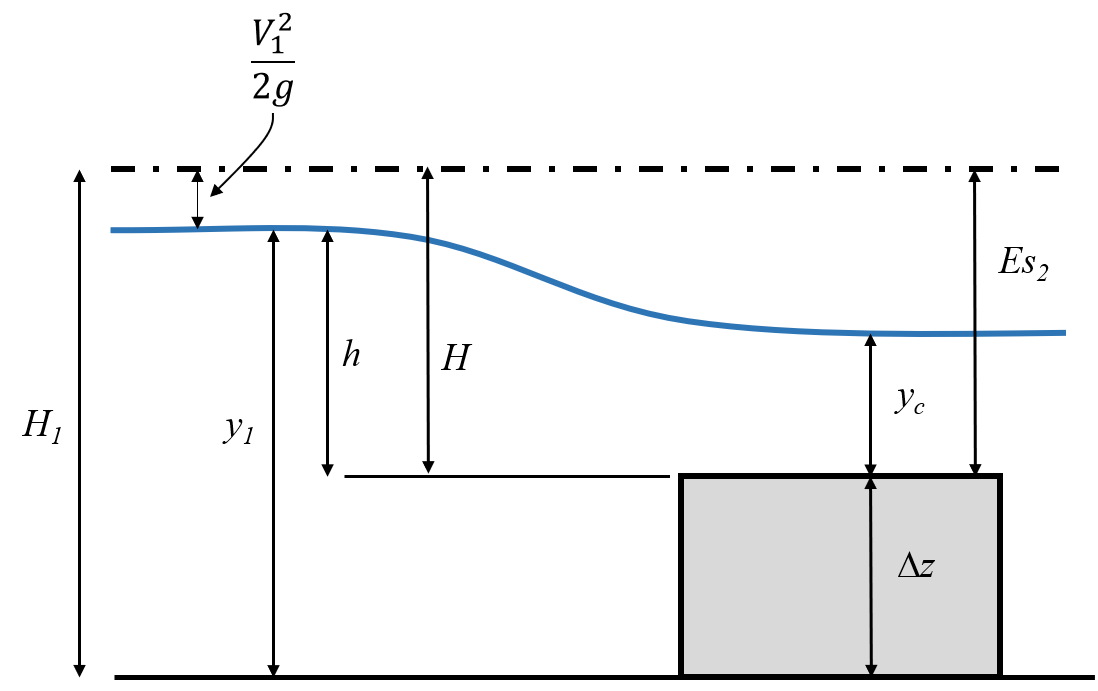
3.1.2 Application of the Specific Energy - Flow over a raised bump

We will look at the example of steady uniform flow that is interrupted by a raised bed level as shown. If the upstream depth, $y_{1}$ , width $B$ and discharge, $Q$ are known we can use the concept of conservation of specific energy - in particular a modification of equation 3.11 with the continuity equation to give the velocity and depth of flow over the raised hump of height $\Delta z$ .

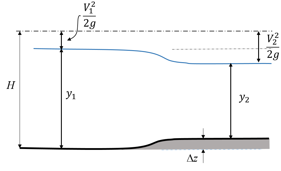
Apply the specific energy between sections 1 and 2. (And assume a horizontal, rectangular channel $z_{1}=z_{2}$ of width $B$ . And take $\alpha=1$ ). The specific energy at point 2 is the flow energy plus the height increase $\Delta z$ :

y_{1}+\frac{V_{1}^{2}}{2g}=y_{2}+\frac{V_{2}^{2}}{2g}+\Delta z

(3.12)

Using the continuity equation

V_{1}A_{1}=V_{2}A_{2}=Q

(3.13)

For a rectangular prismatic channel $A=By$ , so

V_{1}y_{1}=V_{2}y_{2}=\frac{Q}{B}=q

(3.14)

Where $q$ is referred to as the flow per unit width.

Substitute Eqn 3.14 into the Bernoulli equation, Eq 3.12 to give:

y_{1}+\frac{q^{2}}{2gy_{1}^{2}}=y_{2}+\frac{q^{2}}{2gy_{2}^{2}}+\Delta z

(3.15)

rearranging:

y_{2}^{3}+y_{2}^{2}\left(\Delta z-y_{1}-\frac{q^{2}}{2gy_{1}^{2}}\right)+\frac% {q^{2}}{2g}=0

(3.16)

Thus we have the cubic described in the section above, only slightly modified for the bump $\Delta z$ . The only unknown is the downstream depth, $y_{2}$ . Again, there are three solutions to this - only one is correct for this situation. We must find out more about the flow before we can decide which it is.

3.1.3 How Specific Energy, $E_{s}$ changes with depth

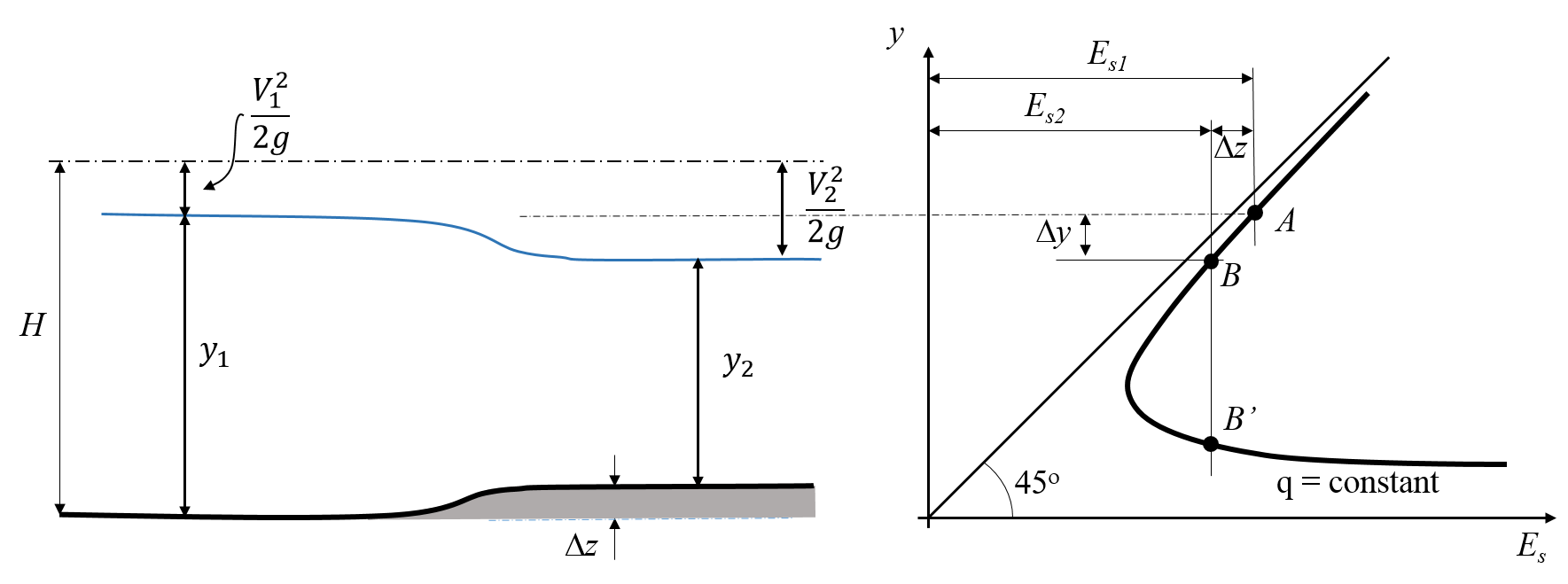
The specific energy equation may be used to solve the raised bump problem. The figure below shows the bump and stage drawn alongside a graph of Specific energy $E_{s}$ against $y$ .

The Specific Energy equation and concept of conservation of energy were applied earlier to this problem and any of these forms of the equation can be written (and are equivalent):

	$\displaystyle E_{s1}$	$\displaystyle=E_{s2}+\Delta z$
	$\displaystyle y_{1}+\frac{V_{1}^{2}}{2g}$	$\displaystyle=y_{2}+\frac{V_{2}^{2}}{2g}+\Delta z$
	$\displaystyle y_{1}+\frac{q^{2}}{y_{1}^{2}2g}$	$\displaystyle=y_{2}+\frac{q^{2}}{y_{2}^{2}2g}+\Delta z$

It is useful to examine figure 3.3 and run horizontal lines from the upstream surface height $y_{1}$ and the height over the bump $y_{2}+\Delta z$ to the $Es\;vs\;y$ curve. Point A on the curve corresponds to the specific energy at point 1 in the channel, but Point B or Point B’ on the graph may correspond to the specific energy at point 2 in the channel.

All points in the channel between points 1 and 2 must lie on the specific energy curve between point A and B or B’. To reach point B’ then this implies that $E_{S1}-E_{S2}>\Delta z$ which is not physically possible. So point B on the curve corresponds to the specific energy and the flow depth at section 2. And point $B^{\prime}$ cannot be physically reached.

Examining the Specific Energy, $Es\;vs\;y$ curve gives us the necessary information to select the correct solution from the cubic equation obtained in these calculations, for example, equation 3.16.

3.1.4 Example of the raised bed hump.

Let’s look at an example calculation to see how this works in practice. A rectangular channel with a flat bed and width $5m$ and maximum depth $2m$ has a discharge of $10m^{3}/s$ . The normal depth is $1.25m$ . What is the depth of flow in a section in which the bed rises $0.2m$ over a distance of $1m$ ?

Assume frictional losses are negligible so we can use this expression

E_{s1}=E_{s2}+\Delta z

Entering the values given in the question

	$\displaystyle E_{s1}$	$\displaystyle=1.25+\frac{\left(\frac{10}{1.25\times 5}\right)^{2}}{2g}=1.38$
	$\displaystyle E_{s2}$	$\displaystyle=y_{2}+\frac{\left(\frac{10}{5\times y_{2}}\right)^{2}}{2g}=y_{2}% +\frac{0.2039}{y_{2}^{2}}$

using

E_{s1}=E_{s2}+\Delta z

	$\displaystyle 1.38$	$\displaystyle=y_{2}+\frac{0.2039}{y_{2}^{2}}+0.2$
	$\displaystyle 1.18$	$\displaystyle=y_{2}+\frac{0.2039}{y_{2}^{2}}=E_{s2}$

This can be solved by a trial and error method with values = $y_{2}$ until the expression is close to $1.18(=E_{s2})$ , for example table 3.1 shows iteration to one of the solutions 0.96m:

Trials of $y_{2}$ $(m)$	$E_{s2}$ $(m$ )
0.9	1.15
1.0	1.2
0.96	1.18

Table 3.1: Trials of

y_{2}

A cubic solver could be used that would give 3 solutions. For this example, these solutions would be $y_{2}=-0.363,\;0.585\;0.958$ .

As the upstream solution is $y_{1}=1.25m$ , and we expect the solution to drop, we know that the highest solution value is the correct one and $y_{2}=0.958m$ . i.e. the depth in the section with the bump is $0.958m$ , that is the the water level (stage) is $1.178m\;(=0.958+0.2)$ a drop of $9cm$ when the bed has been raised $20cm$ .

3.1.5 Flow through a contraction
A Second Application of the Specific energy equation.

Flow through a contraction of the channel is slightly more complex as $q$ is not constant because $b$ is not constant i.e. $b_{1}\neq b_{2}$ so $q_{1}\neq q_{2}\neq q$ . However $Q$ is constant, by continuity.

This means that there are two $Es\;vs\;y$ curves that we must consider, one of $q_{1}$ and on for $q_{2}$ .

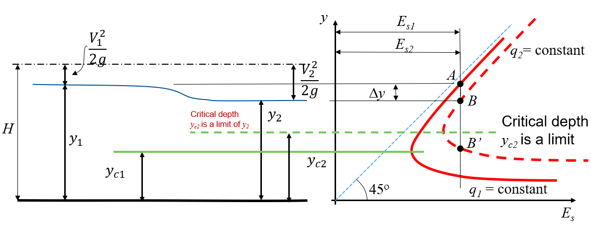
Figure 3.4 shows a figure for these two curves alongside the water surface figure where the corresponding depths in the channel can be seen on these curves.

We see that the specific energy at $y_{1}$ corresponds to point A on the figure - the curve of $q_{1}$ . And a point of the same energy is directly below this at point B, on the $Es\;vs\;y$ curve for $q_{2}$ . Point B’ has the same energy, so would be a solution, but it cannot be reached so it is not physically correct.

This is worthwhile looking at through an example:

Water is flowing at a velocity of $2.3m/s$ and a depth of $3.5m$ in a channel of rectangular section with a width of $3.0m$ . Find the changes in depth produced by a smooth contraction to a width of $2.5m$ .

We have $Q=AV=(3.0\times 3.5)2.3=24.15m^{3}/s$ and thus $q=\frac{Q}{B}=\frac{24.15}{3.0}=8.05m^{3}/s/m$ .

Apply the specific energy equation from point 1 just upstream to point 2 in the converged section (also known as the throat).

E_{s1}=E_{s2}

or

y_{1}+\frac{V_{1}^{2}}{2g}=y_{2}+\frac{V_{2}^{2}}{2g}

or

y_{1}+\frac{Q^{2}}{B_{1}^{2}y_{1}^{2}2g}=y_{2}+\frac{Q^{2}}{B_{2}^{2}y_{2}^{2}% 2g}

or using flow per unit width, $q_{1}=\frac{Q}{B_{1}}$ and $q_{2}=\frac{Q}{B_{2}}$ , then

y_{1}+\frac{q_{1}^{2}}{y_{1}^{2}2g}=y_{2}+\frac{q_{2}^{2}}{y_{2}^{2}2g}

Solve the above for $y_{2}$ given $y_{1}=3.5m,Q=24.15m^{3}/s,B_{1}=3.0m,B_{2}=2.5m$ . We have the cubic

0=y_{2}^{3}-y_{2}^{2}\left(y_{1}+\frac{q_{1}^{2}}{y_{1}^{2}2g}\right)+\frac{q_% {2}^{2}}{2g}

0=y_{2}^{3}-y_{2}^{2}E_{s1}+\frac{q_{2}^{2}}{2g}

We can calculate $E_{s1}=3.77m$ so the cubic equation to solve becomes

0=y_{2}^{3}-3.770y_{2}^{2}+4.756

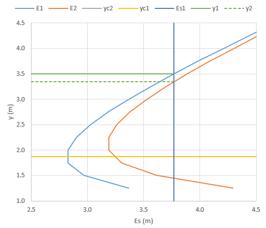
This must be solved using a numerical tool or trial and error to give these 3 solutions $y_{2}=3.344,-0.999,1.424$ .

Figure 3.5 shows the $E_{s}\;vs\;y$ curve for this example with the calculated solution values highlighted. It is clear that $y_{2}=3.344m$ as this is the physical solution (out of the two positive values.)

3.2 Critical, Sub-critical and Super-critical flow

The specific energy change with depth was plotted above for a constant discharge $Q$ , it is also possible to plot a graph with the specific energy fixed and see how $Q$ changes with depth. These two forms are plotted side by side below.

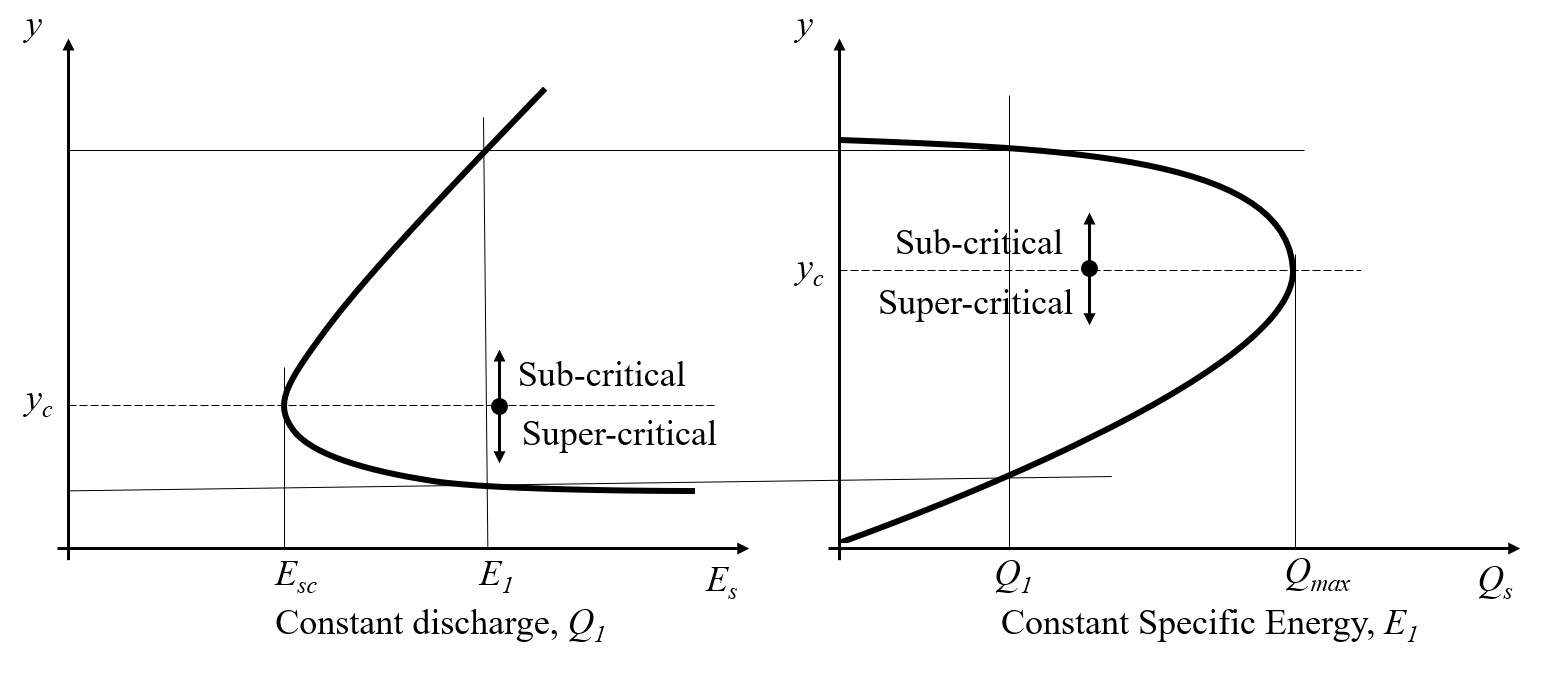
From these graphs, we can identify several important features of rapidly varied flow. For a fixed discharge:

1.

The specific energy is a minimum, $E_{sc}$ , at depth $y_{c}$ ,
This depth is known as critical depth.
2.

For all other values of $E_{s}$ there are two possible depths.
These are called alternate depths (or conjugate depths):

$\displaystyle\textbf{sub-critical flow: }y>y_{c}$

$\displaystyle\textbf{super-critical flow: }y<y_{c}$

For a fixed Specific energy

1.

The discharge is a maximum at critical depth, $y_{c}$ .
2.

For all other discharges there are two possible depths for a particular $E_{s}$
i.e. There is a sub-critical depth and a super-critical depth with the same $E_{s}$ .

An equation for critical depth can be obtained by setting the differential of $E_{s}$ to zero:

E_{s}=y+\frac{(Q/A)^{2}}{2g}

(3.18)

Setting $dE_{s}/dy=0$ gives the turning point

\frac{dE_{s}}{dy}=0=1+\frac{Q^{2}}{2g}\frac{d}{dA}\left(\frac{1}{A^{2}}\right)% \frac{dA}{dy}

(3.19)

Since $\delta A=B\delta y$ , in the limit $dA/dy=B$ and

	$\displaystyle 0$	$\displaystyle=1-\frac{Q^{2}}{2g}B_{c}2A_{c}^{-3}$
	$\displaystyle\frac{Q^{2}B_{c}}{gA_{c}^{3}}$	$\displaystyle=1$		(3.20)

For a rectangular channel $Q=qb$ , $B=b$ and $A=by$ , this equation becomes

y_{c}=\left(\frac{q^{2}}{g}\right)^{1/3}

(3.21)

as $V_{c}y_{c}=q$

V_{c}=\sqrt{gy_{c}}

(3.22)

Substituting this into the specific energy equation

$\displaystyle E_{sc}$	$\displaystyle=y_{c}+\frac{V_{c}^{2}}{2g}$
	$\displaystyle=y_{c}+\frac{y_{c}}{2}$
$\displaystyle y_{c}$	$\displaystyle=\frac{2}{3}E_{sc}$	(3.23)

3.3 Sub and super-critical Flow Determination and Significance

As first introduced in section 1.8, the Froude number is defined for channels as eqn 1.31 and is used primarily to determine whether a flow is sub or super-critical:

F_{r}=\frac{V}{\sqrt{gD_{m}}}

The consideration of specific energy has given us another means of determining whether the flow is sub or super-critical by enabling the calculation of the critical depth: eqn 3.20 in general, or eqn 3.21.

It is worth considering again the significance of sub and super-critical flow.

In super-critical flow, the flow velocity is greater than the wave velocity, so a wave (or any other information about the flow) cannot travel (or influence) upstream. Conversely, the wave can travel upstream in sub-critical flow. i.e. conditions can change upstream in sub-critical flow, but they cannot in super-critical flow.

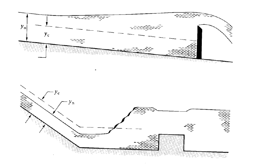
So the value of $F_{r}$ determines the regime of flow - sub, super or critical, and the direction in which disturbances (changes in flow conditions) travel. The summary table from 1.8 is repeated again.

$F_{r}<1$	sub-critical
	water velocity $<$ wave velocity
	upstream levels affected by downstream levels
$F_{r}=1$	critical
$F_{r}>1$	super-critical
	water velocity $>$ wave velocity
	upstream levels NOT affected by downstream levels

Figure 3.7 illustrates this for a flow which is sub-critical (top figure) going over a weir, the raised height of the water moves to affect water upstream. For the (lower figure) super-critical flow down a steep slope forces the flow in the flatter channel downstream.

3.4 Specific Force

While applying momentum principle, Eq. 1.18, for a short horizontal reach of a prismatic channel, one can ignore the external force of friction and the weight component of water for the reach under consideration. If the momentum correction factor $\beta$ is also assumed to be unity [1], (which is valid for a short, prismatic channel), then Eq. 1.18 gives

\rho Q(V_{2}-V_{1})=P_{1}-P_{2}

(3.24)

or

M_{2}-M_{1}=P_{1}-P_{2}

where $M_{1}=\rho QV_{1}$ and $M_{2}=\rho QV_{2}$ , and the hydrostatic forces $P_{1}$ and $P_{2}$ may be expressed as,

P_{1}=\rho g\overline{z}_{1}A_{1}

(3.25)

and

P_{2}=\rho g\overline{z}_{2}A_{2}

(3.26)

Here, $\overline{z}$ represents the distance of the centroid of the flow section $A$ below the free surface. Equation 3.24, therefore, yields or

\rho Q\left(\frac{Q}{A_{2}}-\frac{Q}{A_{1}}\right)=\rho g\overline{z}_{1}A_{1}% -\rho g\overline{z}_{2}A_{2}

or

\frac{Q^{2}}{gA_{1}}+\overline{z}_{1}A_{1}=\frac{Q^{2}}{gA_{2}}+\overline{z}_{% 2}A_{2}

(3.27)

Both sides of Eq. 3.27 are similar and, hence, may be expressed as, say,

F=\frac{Q^{2}}{gA}+\overline{z}A

(3.28)

Here, the term $Q^{2}/gA$ is the momentum of the flow (i.e. $\rho QU$ or $\rho Q^{2}/A$ ) passing through a flow section of a channel per unit time per unit weight of the flowing fluid. The second term on the right side of Eq. 3.28, $\overline{z}A$ represents the hydrostatic force per unit weight of water. Thus, $F$ is essentially the sum of the two forces per unit weight of water and, therefore, called the specific force. Equation 3.27 can, accordingly, be written as

F_{1}=F_{2}

meaning that the specific forces at the end sections of a channel reach is equal provided that the channel is horizontal (or the bed slope of the channel is very small) and the external forces (e.g. friction) acting on the flowing fluid between the end sections can be ignored.

3.5 Application of the Momentum equation for Rapidly Varied Flow

3.5.1 Force on Structure in Open Channel Flow

If we consider an obstruction (which could represent any structure, bridge, gate etc.) in a flow, such as that shown in figure 3.8, we analyse the forces on that obstruction by considering a control volume - such as that shown as a dashed box and consider the momentum change entering and leaving the control volume. (For a short length of channel over a structure, it is common and appropriate to neglect the forces due to the fluid weight and frictional resistance). The rate of change of the momentum gives the Total force or Momentum force, $M$ .

	$\displaystyle M$	$\displaystyle=\rho QV_{2}-\rho QV_{1}$
		$\displaystyle=M_{2}-M_{1}$
		$\displaystyle=\rho Q(V_{2}-V_{1})$

The Pressure force $P$ is

	$\displaystyle P$	$\displaystyle=\rho g\overline{z}_{1}A_{1}-\rho g\overline{z}_{2}A_{2}$
		$\displaystyle=P_{1}-P_{2}$
		$\displaystyle=\rho g(\overline{z}_{1}A_{1}-\overline{z}_{2}A_{2})$

For a rectangular channel, where $\overline{z}=\frac{y}{2}$ and $A=by$ , then

P=\rho gb\frac{1}{2}(y^{2}_{1}-y^{2}_{2})

We can equate the total force to the pressure plus reaction force, $F_{R}$ , the force the structure exerts on the fluid. (The force that the fluid exerts on the structure is equal in magnitude but in the opposite directions, i.e. $R=-F_{R}$ .)

	$\displaystyle M$	$\displaystyle=P+F_{R}$
	$\displaystyle R=-F_{R}$	$\displaystyle=P-M$
		$\displaystyle=\left(\rho QV_{1}+\rho g\overline{z}_{1}A_{1}\right)-\left(\rho QV% _{2}+\rho g\overline{z}_{2}A_{2}\right)$

and for a rectangular channel

R=-F_{R}=\left(\rho QV_{1}+\rho gb\frac{y^{2}_{1}}{2}\right)-\left(\rho QV_{2}% +\rho gb\frac{y^{2}_{2}}{2}\right)

(3.29)

3.5.2 Analysis of the Hydraulic Jump Using the Momentum Equation

The hydraulics jump is an important feature in open channel flow and is an example of rapidly varied flow. A hydraulic jump occurs when a super-critical flow and a sub-critical flow meet. The jump is the mechanism for the surfaces at the lower and upper levels to join. They join in an extremely turbulent manner which causes large energy losses.

Because of the large energy losses the energy or specific energy equation cannot be used in analysis, the momentum equation is used instead.

\text{Resultant pressure force in }x-\text{direction}=P_{1}-P_{2}

\text{Rate of Momentum change }=M_{2}-M_{1}

M_{2}-M_{1}=P_{1}-P_{2}

Or for a constant discharge

M_{2}-M_{1}=P_{1}-P_{2}=\text{constant}

For a rectangular channel, we can write these expressions (following section 3.5.1 above) as

\begin{aligned} P_{1}&=\rho g\frac{y_{1}}{2}y_{1}b\\ M_{1}&=\rho QV_{1}\\ &=\rho Q\frac{Q}{y_{1}b}\end{aligned}\qquad\qquad\begin{aligned} P_{2}&=\rho g% \frac{y_{2}}{2}y_{2}b\\ M_{2}&=\rho QV_{2}\\ &=\rho Q\frac{Q}{y_{2}b}\end{aligned}

Substituting for these and rearranging gives

y_{2}=\frac{y_{1}}{2}\left(\sqrt{1+8F_{r1}^{2}}-1\right)

(3.30)

Or

y_{1}=\frac{y_{2}}{2}\left(\sqrt{1+8F_{r2}^{2}}-1\right)

(3.31)

Thus, knowing the discharge and either one of the depths on the upstream or downstream side of the jump, the other - or sequent (or conjugate or alternate) depth - may be easily computed.

More manipulation of Equation 3.30 and the specific energy equation gives the energy loss in the jump as

\Delta E=\frac{(y_{2}-y_{1})^{3}}{4y_{1}y_{2}}

(3.32)

These are useful results in particular for gradually varied flow calculations to determine water surface profiles enabling detection and positioning of hydraulic jumps.

In summary, a hydraulic jump will only occur if the upstream flow is super-critical. The higher the upstream Froude number the higher the jump and the greater the loss of energy in the jump.

3.6 Rapidly varied flow and Critical-depth structures

The effect of a local rise in the bed level on the flow has been discussed earlier. It was shown that the depth would fall as the flow went over the rise. If this rise were large enough (for the particular velocity) the fall would be enough to give critical depth over the rise. Increasing the rise further would not decrease the depth but it would remain at critical depth. This observation may be confirmed by studying further the specific energy equation in a similar way to earlier.

The fact that depth is critical over the rise and that critical depth can be calculated quite easily for a given discharge is made use of in hydraulic structures for flow measurement. Actually, it is the converse of the above, that the discharge can be easily calculated if the critical depth is known, that is most useful.

3.6.1 Broad-crested weir

Assuming that the depth is critical over the rise then we know

V_{2}=V_{c}=\sqrt{gy_{c}}

Q=AV_{c}=by_{c}\sqrt{gy_{c}}

where $b$ is the width of the channel

Earlier it was shown in Eqn 3.23 that

y_{c}=\frac{2}{3}E_{sc}

Assuming no energy loss between 1 and 2

	$\displaystyle E_{s_{2}}$	$\displaystyle=h+\frac{V_{1}^{2}}{2g}=H$
	$\displaystyle y_{c}$	$\displaystyle=\frac{2}{3}H$

So

	$\displaystyle Q$	$\displaystyle=\frac{2}{3}\sqrt{\frac{2g}{3}}bh^{3/2}$
		$\displaystyle=1.705bh^{3/2}$

in practice, there are energy losses upstream of the weir. To incorporate this a coefficient of discharge and of velocity are introduced to give

Q=C_{d}C_{v}1.705bh^{3/2}

(3.33)

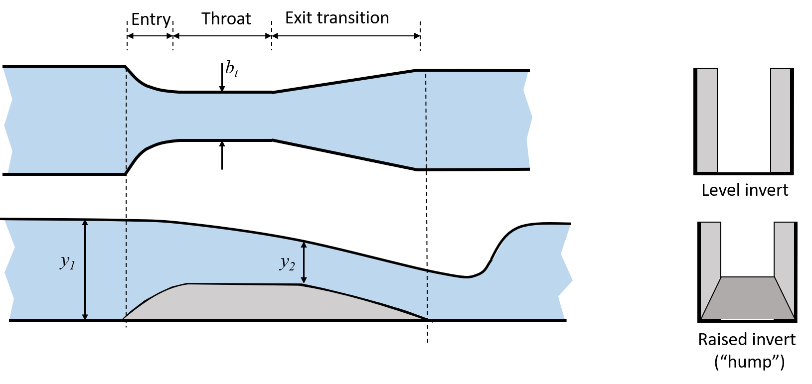
3.6.2 Flumes

A second method of measuring flow by causing critical depth is to contract the flow. Similar specific energy arguments to those used for a raised bed can be used in the analysis of this situation, and they come to similar predictions that depth will fall and not fall below critical depth.

It is also possible to combine the two by putting a raised section within the narrowed section.

These types of structures are known as flume, and the first type is known as a Venturi flume.

3.6.3 Venturi flume

Flumes are usually designed to achieve critical depth in the narrowest section (the throat) while also giving a very small afflux.

The general equation for the ideal discharge through a flume can be obtained from the energy and continuity considerations.

The energy equation gives:

E_{s}=y_{1}+\frac{V_{1}^{2}}{2g}=y_{2}+\frac{V_{2}^{2}}{2g}

by continuity $V_{1}=Q/(by_{1})$ and $V_{2}=Q/(b_{2}y_{2})$

which when substituted into the energy equation gives

Q=by_{1}\sqrt{\frac{2g(y_{1}-y_{2})}{[(by_{1})/(b_{2}y_{2})]^{2}-1}}

If critical flow is achieved in the throat then $y_{2}=\frac{2}{3}E_{s}$ which can be substituted to give (in SI units)

Q=1.705b_{2}E_{s}^{3/2}

or introducing a velocity correction factor and a discharge coefficient

Q=1.705b_{2}C_{v}C_{d}y_{1}^{3/2}

(3.34)

	$\displaystyle\textbf{sub-critical flow: }y>y_{c}$
	$\displaystyle\textbf{super-critical flow: }y<y_{c}$

3 Rapidly Varied Flow