2 Uniform Flow in Open Channels

2.1 Uniform flow and the Development of Friction formulae

When uniform flow occurs gravitational forces exactly balance the frictional resistance forces which apply as a shear force along the boundary (channel bed and walls).

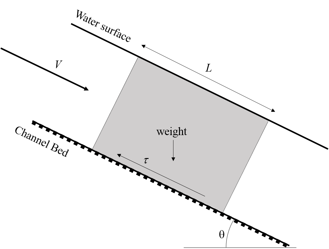
Refer to caption — Figure 2.1: Forces on a channel length in uniform flow

Considering figure 2.1, the gravity force resolved in the direction of flow is

\text{gravity force}=\rho gAL\sin\theta

(2.1)

and the boundary shear force resolved in the direction of flow is

\text{shear force}=\tau_{o}PL

(2.2)

In uniform flow these balance

\tau_{o}PL=\rho gAL\sin\theta

(2.3)

Considering a channel of small slope, then

\sin\theta\approx\tan\theta=S_{o}

(2.4)

\tau_{o}=\frac{\rho gAS_{o}}{P}=\rho gRS_{o}

(2.5)

2.1.1 The Chezy equation

If an estimate of $\tau_{o}$ can be made then we can make use of Equation 2.5.

If we assume the state of rough turbulent flow then we can also make the assumption the shear force is proportional to the flow velocity squared i.e.

	$\displaystyle\tau_{o}$	$\displaystyle\propto V^{2}$
	$\displaystyle\tau_{o}$	$\displaystyle=KV^{2}$

Substituting this into equation 2.5 gives

V=\sqrt{\frac{\rho g}{K}RS_{o}}

(2.6)

Or grouping the constants together as one equal to $C$

V=C\sqrt{RS_{o}}

(2.7)

This is the Chezy equation and the $C$ the ’Chezy $C$ ’

In terms of $Q(=AV)$ this is simply

Q=AC\sqrt{RS_{o}}

(2.8)

Because the $K$ is not constant the $C$ is not constant but depends on Reynolds number and boundary roughness (see discussion in previous section).

Although not a specific practical use, as a purely technical interest, the relationship between $C$ and $\tau$ can easily be seen by substituting equation 2.7 into the Darcy-Wiesbach equation written for open channels to show

C=\sqrt{\frac{2g}{f}}

(2.9)

2.2 The Manning’s equation

Very many studies have been made on the evaluation of C for different natural and man-made channels. These have resulted in today where most practising engineers use some form of this relationship to give $C$ :

C=\frac{R^{1/6}}{n}

(2.10)

This is known as Manning’s formula, or the Manning’s equation, and the $n$ as Manning’s $n$ .

Substituting equation 2.10 in to 2.7 gives velocity of uniform flow:

V=\frac{1}{n}R^{2/3}S_{o}^{1/2}

(2.11)

Or in terms of discharge

Q=\frac{1}{n}AR^{2/3}S_{o}^{1/2}

(2.12)

Or as $R=A/P$

Q=\frac{1}{n}\frac{A^{5/3}}{P^{2/3}}S_{o}^{1/2}

(2.13)

Either of equations 2.12 or 2.13 we will refer to as the Manning’s equation.

Note:
Several other names have been associated with the derivation of this formula - or ones similar and consequently, in some countries the same equation is named after one of these people. Some of these names are; Strickler, Gauckler, Kutter, Gauguillet and Hagen. See for example this informative web page https://en.wikipedia.org/wiki/Manning_formula.

The Manning’s $n$ is also numerically identical to the Kutter $n$ .

Manning’s equation has the great benefit that it is simple and accurate, and now, due to its long extensive practical use, there exists a wealth of publicly available values of $n$ for a very wide range of channels.

Below is a table of a few typical values of Manning’s $n$

Channel type	Surface material and form	Manning’s $n$ range
River	earth, straight	0.02-0.025
	earth, meandering	0.03-0.05
	gravel (75-150mm), straight	0.03-0.04
	gravel (75-150mm), winding	0.04-0.08
unlined canal	earth, straight	0.018-0.025
	rock, straight	0.025-0.045
lined canal	concrete	0.012-0.017
lab. models	mortar	0.011-0.013
	Perspex	0.009

Table 2.1: Table of Manning’s n values for common channel material

Appendix A has further details of the Manning’s equation written in different forms as well as for commonly shaped channels: rectangular, trapezoidal, circular and wide. It is very important that you look at this appendix.

2.2.1 Conveyance

Channel conveyance, $K$ , is a measure of the carrying capacity of a channel. The $K$ is really an agglomeration of several terms in the Chezy or Manning’s equation:

	$\displaystyle Q$	$\displaystyle=AC\sqrt{RS_{o}}$
		$\displaystyle=KS_{o}^{1/2}$		(2.14)

K=ACR^{1/2}=\frac{1}{n}\frac{A^{5/3}}{P^{2/3}}=\frac{1}{n}AR^{2/3}

(2.15)

The use of conveyance is sometimes convenient when calculating discharge and stage in compound channels (e.g. channels with a main channel and a flood plain) and also calculating the energy and momentum coefficients in this situation.

2.3 Computations in uniform flow

We can use either the Chezy or Manning’s equations for discharge to calculate steady uniform flow. Two calculations are usually performed to solve uniform flow problems.

1.

Discharge from a given depth
2.

Depth for a given discharge

In steady uniform flow the flow depth is known as normal depth.

We will continue the discussion based on the Manning’s equation, as that is the most common in practise. However all uniform flow computations described in the following text could also be done using the Chezy equation (with an appropriate Chezy C prescribed).

As we have already mentioned, and by definition, uniform flow can only occur in channels of constant cross-section (prismatic channels) so natural channels can be excluded. However we will need to use Manning’s equation later for gradually varied flow in natural channels - so application to natural/irregular channels will often be required.

2.3.1 Uniform flow example 1 - Discharge from depth in a trapezoidal channel

A concrete-lined trapezoidal channel with uniform flow has a normal depth of 2m. The base width is $5m$ and the side slopes are equal at 1:2 (v:h, or $s=2$ in table 1.2) Manning’s $n$ can be taken as $0.015$ , And the bed slope $S_{o}=0.001$

What are:

a)

Discharge ( $Q$ )?
b)

Mean velocity ( $V$ )?
c)

Reynolds number ( $R_{e}$ )?

Calculate the section properties, using the appropriate geometrical formulae (e.g. table 1.2)

Area, $A=(b+sy)y$

A=(5+2y)y=18m^{2}

Wetted perimeter, $P=b+2y\sqrt{1+s^{2}}$

P=5+2y\sqrt{1+2^{2}}=13.94m

Use equation 2.13 to get the discharge

	$\displaystyle Q$	$\displaystyle=\frac{1}{n}\frac{A^{5/3}}{P^{2/3}}S_{o}^{1/2}$
		$\displaystyle=\frac{1}{0.015}\frac{18^{5/3}}{13.94^{2/3}}0.001^{1/2}$
		$\displaystyle=45m^{3}/s$

Calculate the mean velocity using the continuity equation:

V=\frac{Q}{A}=\frac{45}{18}=2.5m/s

And the Reynolds, $R_{e}$ , number (remember we use the hydraulic radius $R$ as the length scale), and so using $R=A/P$ )

R_{e}=\frac{\rho VR}{\mu}=\frac{\rho V}{\mu}\frac{A}{P}=\frac{1000\times 2.5}{% 1.14\times 10^{-3}}\frac{18}{13.9}=2.84\times 10^{6}

This is very large - i.e. well into the turbulent zone - the application of the Manning’s equation was therefore valid.

What solution would we have obtained if we had used the Colebrook-White equation which takes into account the changes in roughness with $Re$ ?

The likely hood is that results would be very very similar (negligibly so) as, looking at the $Re$ , we are well into the rough-turbulent zone where a constant friction value is truly applicable.

To investigate further with the Colebrook-White equation, an equivalent $k_{s}$ value can be calculated for the discharge obtained from $n=0.015$ and $y=2m$ [ $k_{s}=2.225mm$ ] (Using the Colebrook-White equation and the Darcy-Wiesbach equation of open channels - both given earlier). Then a range of depths can be chosen and the discharges calculated for these $n$ and $k_{s}$ values. Comparing these discharge calculations will give some idea of the relative differences - they will be very similar.

2.3.2 Uniform flow example 2 - Depth from Discharge in a trapezoidal channel

Using the same channel as above, if the discharge is known to be $30m^{3}/s$ in uniform flow, what is the normal depth?

Again use equation 2.13

Q=\frac{1}{n}\frac{A^{5/3}}{P^{2/3}}S_{o}^{1/2}

And substituting using
Area, $A=(b+sy)y$
Wetted perimeter, $P=b+2y\sqrt{1+s^{2}}$

	$\displaystyle Q$	$\displaystyle=\frac{1}{0.015}\frac{((5+2y)y)^{5/3}}{\left(2+2y\sqrt{1+2^{2}}% \right)^{2/3}}0.001^{1/2}$
	$\displaystyle 30$	$\displaystyle=2.108\frac{((5+2y)y)^{5/3}}{\left(2+2y\sqrt{1+2^{2}}\right)^{2/3}}$

We need to calculate $y$ from this equation (and remember that this is normal depth so $y=y_{n}$ .

Even for this quite simple geometry, the equation we need to solve for normal depth is complex (and not explicit).

One simple strategy to solve this is to try some trial values of $y$ and calculate the right-hand side of this equation and compare it to $Q(=30m^{3}/s)$ on the left. When it equals $Q$ we have the correct $y$ . Even though there will be several solutions to this equation, this strategy generally works because we have a good idea of what the depth should be (e.g. it will always be positive and often in the range of $0.5\text{ to }10m$ ).

In this case from the previous example, we know that at $Q=45m^{3}/s$ , $y=2m$ . So at $Q=30m^{3}/s$ then $y<2.0m$ .

Trials of $y$ ( $m$ )	Discharge $Q$ ( $m^{3}/s$ )
1.7	32.7
1.6	29.1
1.63	30.1

Table 2.2: Trials of

y

2.3.3 Uniform flow example 3 - Calculation of Uniform Flow and Froude Number

Find the discharge in the channel shown in figure 2.2 that is flowing with uniform flow of depth $4m$ , as shown below, and has a bed slope $S_{o}$ is 1 in 1000 and a Chezy $C$ of $45m^{1/2}/s$ . Is this flow sub or super-critical?

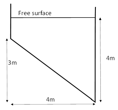
We have uniform flow and the friction is specified by the Chezy $C$ friction factor, so use the Chezy Equation (equation 2.8):

Q=AC\sqrt{RS_{o}}

Slope: $S_{o}=1/1000=0.001v$

Flow area: $A=((3\times 4))/2+1\times 4=10m^{2}$

Wetted perimeter: $P=1+sqrt{3^{2}+4^{2}}+4=10m$

Hydraulic radius: $R=A/P=1m$

Hydraulic mean depth: $D_{m}=A/B=10/4=2.5m$

Therefore the discharge in the channel is $Q=10\times 45\sqrt{1\times 0.001}=14.23m^{3}/s$

And the velocity of flow is $V=Q/A=14.23/10=1.423m/s$

To calculate whether the flow is sub or super-critical then we must calculate the Froude number $F_{r}$ using equation 1.31.

Fr=\frac{V}{gD_{m}}=\frac{1.423}{9.8\times 2.5}=0.287

As $F_{r}<1$ , it is sub-critical flow.

2.3.4 Uniform flow example 4 - A compound channel

The channel shown in figure 2.3 has been designed so that usually the water flows in the lower trapezoidal section in the middle (region 1). During high flow conditions (e.g. flooding) the water level will rise above this and will be flowing across the full section including the two floodplains of regions 2 and 3.

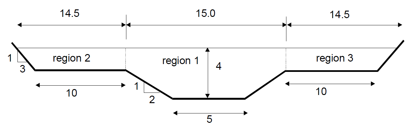
With the flood channels dimensions as shown and the Manning $n$ in the main channel and on the banks estimated as $0.015$ and $0.035$ respectively, what is

a)

the discharge for a flood level of $4m$ (measured from the lowest point of the cross-section)?
b)

the energy coefficient $\alpha$ ?

First, split the section as shown into three regions (this is arbitrary and left to the engineers’ judgment). Then apply Manning’s formula for each section to give three discharge values and the total discharge will be $Q=Q_{1}+Q_{2}+Q_{3}$ .

Calculate the properties of each region:

A_{1}=\left(\frac{5+15}{2}\right)2.5+(15\times 1.5)=47.5m^{2}

A_{2}=A_{3}=\left(\frac{10+14.5}{2}\right)1.5=18.38m^{2}

P_{1}=5+\left(2\sqrt{5}\times 2.5\right)=16.18m

P_{2}=P_{3}=10+\left(1.5\sqrt{10}\times\right)=14.75m

The conveyance for each region may be calculated from equation 2.15

K_{1}=\frac{47.5^{5/3}}{0.015\times 16.18^{2/3}}=6492.5

K_{2}=K_{3}=\frac{18.38^{5/3}}{0.035\times 14.74^{2/3}}=608.4

And from Equation 2.13 or Equation 2.14 the discharges

Q_{1}=\frac{1}{0.015}\frac{47.5^{5/3}}{16.18^{2/3}}0.001^{1/2}

Q_{1}=K_{1}0.001^{1/2}=205.3m^{3}/s

And

Q_{2}=Q_{3}=\frac{1}{0.035}\frac{18.38^{5/3}}{14.74^{2/3}}0.001^{1/2}

Q_{2}=Q_{3}=K_{2}0.001^{1/2}=19.2m^{3}/s

Q=Q_{1}+Q_{2}+Q_{3}=243.7m^{3}/s

The velocities can be obtained from the continuity equation:

V_{1}=\frac{Q_{1}}{A_{1}}=4.32m/s

V_{2}=V_{3}=\frac{Q_{2}}{A_{2}}=1.04m/s

And the energy coefficient may be obtained from Equation 1.15

\alpha=\frac{\int u^{3}\;dA}{\overline{V}^{3}\;A}=\frac{V_{1}^{3}A_{1}+V_{2}^{% 3}A_{2}+V_{3}^{3}A_{3}}{\overline{V}^{3}(A_{1}+A_{2}+A_{3})}

where

\overline{V}=\frac{Q}{A}=\frac{V_{1}A_{1}+V_{2}A_{2}+V_{3}A_{3}}{A_{1}+A_{2}+A% _{3}}

Giving

\alpha=1.9

This is a very high value of $\alpha$ and a clear case of where a velocity coefficient should be used.

Note that this method does not give a completely accurate relationship between stage and discharge because some of the assumptions are not accurate. E.g. the arbitrarily splitting into regions of fixed Manning $n$ is probably not what is occurring in the actual channel. However, it will give a good estimate as long as care is taken in choosing these regions.

2.4 Efficient Uniform Flow Channels

The design of a rigid (i.e., non-erodible) surface open channel should be such that it is capable of carrying maximum discharge with minimum excavation, construction, and lining costs. This suggests minimising the friction which also suggests that the designed channel should have a maximum hydraulic radius for a given area or minimum perimeter for the given area since hydraulic radius equals $A/P$ . Therefore, a circular or semi-circular cross-section is the most efficient section. The use of a circular channel section is usually not feasible for sections larger than when a pipe could be used, due to the difficulties of construction to achieve stable earth slopes and other practical considerations. Hence, the designer has to determine the most efficient section of a given shape. Considering a trapezoidal channel section, Fig. 2.4, the area of flow section $A$ and the wetted perimeter $P$ are given as

A=by+sy^{2}

(2.16)

P=b+2y\sqrt{1+s^{2}}

(2.17)

Here,

s=\cot\theta\qquad\qquad\text{or }\qquad\qquad\frac{1}{s}=\tan\theta

On substituting the value of $b$ obtained from Eq. 2.16 into Eq. 2.17, one gets

P=\frac{A}{y}-sy+2y\sqrt{1+s^{2}}

(2.18)

To minimize $P$ , evaluate $dP/dy$ with $A$ and $s$ constant and set $dP/dy$ equal to zero. Therefore,

\frac{dP}{dy}=-\frac{A}{y^{2}}-s+2\sqrt{1+s^{2}}=0

A=y^{2}\left[2\sqrt{1+s^{2}}-s\right]

(2.19)

Substituting the expression for $A$ into Eq. 2.16, one gets

by+sy^{2}=y^{2}\left[2\sqrt{1+s^{2}}-s\right]

$\therefore$

b=2y\left[\sqrt{1+s^{2}}-s\right]

(2.20)

Likewise, substituting the value of $A$ from Eq. 2.19 in Eq. 2.18, one gets

P_{min}=y\left[2\sqrt{1+s^{2}}-s\right]-sy+2y\sqrt{1+y^{2}}

P_{min}=4y\sqrt{1+s^{2}}-2sy=2y\left[2\sqrt{1+s^{2}}-s\right]

(2.21)

Thus,

R_{optimum}=\frac{A}{P}=\frac{y}{2}

(2.22)

Equation 2.22 indicates that for any side slope $\theta$ (or $s$ ), the most efficient uniform flow channel of trapezoidal shape would be the one for which the hydraulic radius is half the depth of flow.

For a rectangular section, $\theta=$ 90 or $s=$ 0. Therefore, the most efficient rectangular channel section would be the one for which

A=2y^{2}

P=4y

R=y/2

B=2y

To obtain the depth of flow for the most efficient section, these equations must be solved in conjunction with the Manning’s equation.

Equations 2.19, 2.22 are valid for any value of $s$ . The best value of $s$ for given $y$ and $A$ can be obtained by setting $dP/ds$ , evaluated from Eq. 2.18, equal to zero.

\frac{dP}{ds}=-y+2y\left[\frac{1}{2}\frac{1}{\sqrt{1+s^{2}}}\right]2s=0

$\therefore$

2s=\sqrt{1+s^{2}}

$\therefore$

s=\frac{1}{\sqrt{3}}=\cot\theta\qquad\qquad\text{or}\qquad\qquad\frac{1}{s}=% \tan\theta=\sqrt{3}

$\therefore$

\theta=60^{\circ}

Thus, the maximum-flow trapezoidal section would be half of a hexagon.

Similarly, one can show that a circular channel section running partially full would perform best when the depth of flow is half the diameter. Geometric elements of the most efficient channel sections of some selected shapes are given in Table 2.3. Obviously, the semi-circular open channel section is the best of all possible channel sections as it gives the minimum wetted perimeter for a given area of flow section. However, the percentage increase in discharge for semicircular section, compared to that in semi-hexagonal section is only small.

Cross-section	Normal	Area,	Wetted	Hydraulic	Water surface	Hydraulic
	depth, $y_{n}$	$A$	perimeter, $P$	radius, $R$	width, $B$	depth, $D$
Rectangular	$0.917(Qn/\sqrt{S})^{3/8}$	$2y^{2}$	$4y$	$0.500y$	$2y$	$y$
Triangle	$1.297(Qn/\sqrt{S})^{3/8}$	$y^{2}$	$2.83y$	$0.354y$	$2y$	$0.500y$
(side slope 1:1)
Trapezoid	$0.968(Qn/\sqrt{S})^{3/8}$	$1.73y^{2}$	$3.46y$	$0.500y$	$2.31y$	$0.750y$
(half of a hexagon)
Semicircle	$1.000(Qn/\sqrt{S})^{3/8}$	$0.5\pi y^{2}$	$\pi y$	$0.500y$	$2y$	$0.250\pi y$
Parabola	$0.937(Qn/\sqrt{S})^{3/8}$	$1.89y^{2}$	$3.77y$	$0.500y$	$2.83y$	$0.667y$
$B=2\sqrt{2y}$

Table 2.3: Geometric elements of the most efficient hydraulic sections [3]