1 Basic Equations of Open Channel Hydraulics ‣ CIVE3415: Water Engineering III Steady Open Channel Hydraulics

1.1 Definition and differences between pipe flow and open channel flow

The flow of water in a conduit may be either open channel flow or pipe flow. The two kinds of flow are similar in many ways but differ in one important respect. Open-channel flow must have a free surface, whereas pipe flow has none. A free surface is subject to atmospheric pressure. Pipe flow exerts no direct atmospheric flow but hydraulic pressure only.

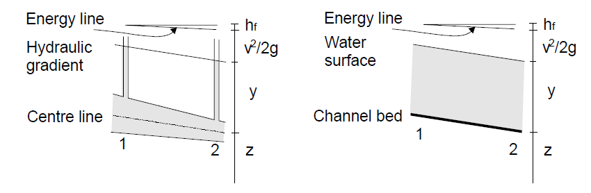
Refer to caption — Figure 1.1: Figure of pipe and open channel flow

The two kinds of flow are compared in the figure above. On the left is pipe flow. Two piezometers are placed in the pipe at sections 1 and 2. The water levels in the pipes are maintained by the pressure in the pipe at elevations represented by the hydraulics grade line or hydraulic gradient. The pressure exerted by the water in each section of the pipe is shown in the tube by the height y of a column of water above the centre line of the pipe.

The total energy of the flow of the section (with reference to a datum) is the sum of the elevation z of the pipe centre line, the piezometric head y and the velocity head $V^{2}/2g$ , where $V$ is the mean velocity. The energy is represented in the figure by what is known as the energy grade line or the energy gradient. The loss of energy that results when water flows from section 1 to section 2 is represented by $h_{f}$ .

A similar diagram for open channel flow is shown to the right. This is simplified by assuming parallel flow with a uniform velocity distribution and that the slope of the channel is small. In this case, the hydraulic gradient is the water surface as the depth of water corresponds to the piezometric height.

Despite the similarity between the two kinds of flow, it is much more difficult to solve problems of flow in open channels than in pipes. Flow conditions in an open channel are complicated by the position of the free surface which is likely to change with time and space. And also the fact that depth of flow, the discharge, and the slopes of the channel bottom and of the free surface are all interdependent.

Physical conditions in open channels vary much more than in pipes - the cross-section of pipes is usually round - but for open channels it can be any shape.

Treatment of roughness also poses a greater problem in open channels than in pipes. Although there may be a great range of roughness in a pipe from polished metal to highly corroded iron, open channels may be of polished metal to natural channels with long grass and roughness that may also depend on the depth of flow.

Open channel flows are found in large and small scales. For example, the flow depth can be between a few $cm$ in water treatment plants and over $10m$ in large rivers. The mean velocity of flow may range from less than $0.01m/s$ in tranquil waters to above $50m/s$ in high-head spillways. The range of total discharges may extend from $0.001l/s$ in chemical plants to greater than $10000m^{3}/s$ in large rivers or spillways.

In each case the flow situation is characterised by the fact that there is a free surface whose position is NOT known beforehand - it is determined by applying momentum and continuity principles.

In general, the treatment of open-channel flow is more empirical than pipe flow - but can still produce useful results.

Open channel flow is driven by gravity in most cases rather than by pressure work as in pipes.

Table 1.1: Differences Between Pipe Flow and Open Channel Flow

	Pipe Flow	Open Channel Flow
Flow driven by	Pressure work	Gravity (potential energy)
Flow cross-section	Known, fixed	Unknown in advance because the flow depth is unknown
Characteristic flow parameters	velocity deduced from continuity	Flow depth deduced simultaneously from solving both continuity and momentum equations
Specific boundary conditions		Atmospheric pressure at the free surface

1.2 Types of flow / Classification of flow

Open-channel flow is steady if all flow properties are independent of time. The most important examples of unsteady flow are waves, surges and tidal flows.

In this part of the course, we consider only steady flow. For a given channel this consists of various fetches considered as uniform flow.

The classifications discussed below are made according to changes in flow depth with respect to time and space.

•

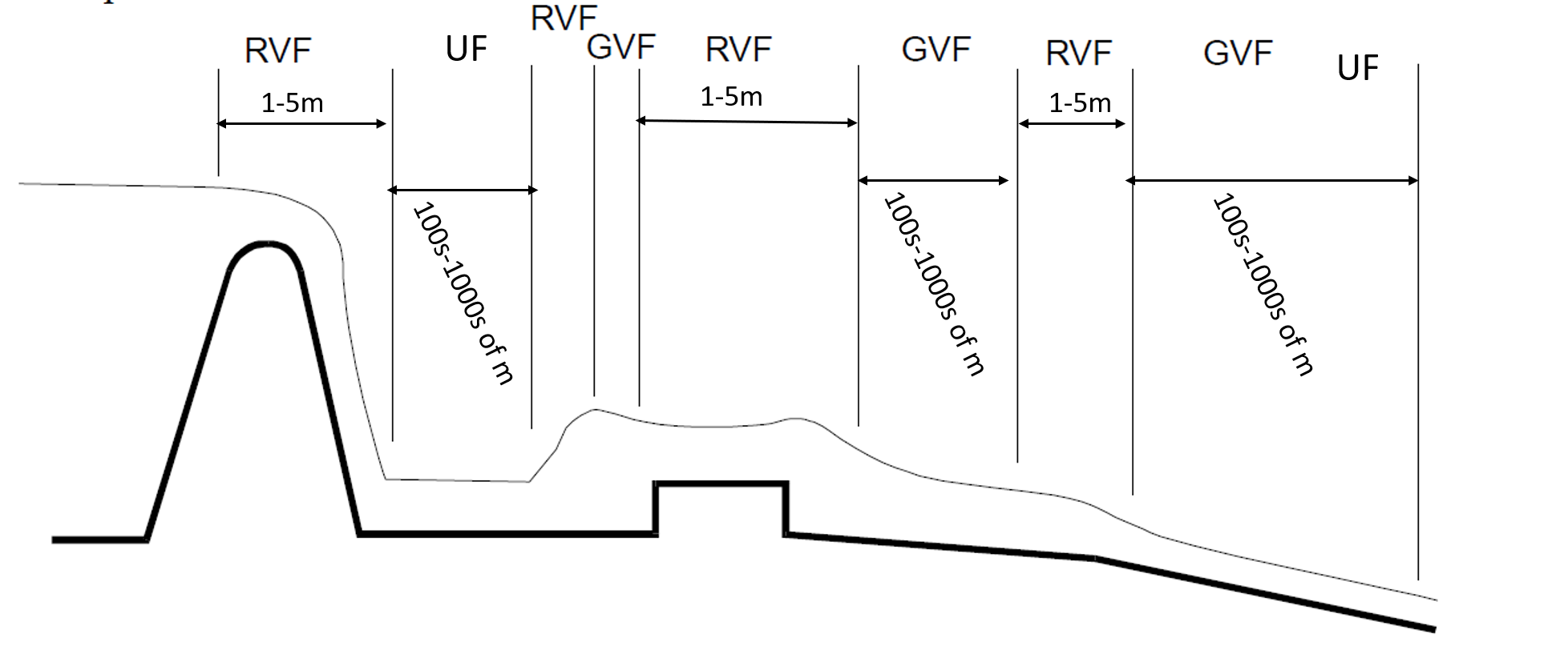
Uniform flow, UF
In uniform flow, the depth and cross-stream velocity profile does not vary in the direction of flow. This can only occur in a long straight channel of uniform cross-section, constant slope and no side streams. (These are called prismatic channels; they are always an approximation when considering natural water courses like rivers). Here, the downslope component of weight exactly balances bed friction. The depth in steady uniform flow is called normal depth (and hence the flow is sometimes referred to as normal flow). All steady downslope flow in prismatic channels tends to uniform flow, and thus normal depth, if there is sufficient undisturbed distance.
•

Rapidly Varied Flow, RVP
Rapidly-varied flow occurs when the flow adjusts over relatively short distances (a few times the flow depth). Examples are hydraulic jumps, as well as flow past hydraulic structures such as weirs, venturis (local narrowing) and sluices. Because the streamwise distance is relatively short, the rapid changes to flow properties can often be obtained by neglecting bed friction.
•

Gradually Varied Flow, GVF
In gradually-varied flow the water depth changes slowly with streamwise distance (typically over distances of hundreds or thousands of times the flow depth) because of an imbalance between gravitational and friction forces. This may occur as the result of a change in channel conditions (slope, cross-section or roughness) or as an adjustment brought about by upstream or downstream disturbances such as weirs and sluices. Because the variation is gradual the flow can still be treated as one-dimensional (varying only with $x$ ) and the pressure as hydrostatic.

1.3 Properties of open channels

Artificial channels
These are channels made by humans. They include canals, navigation canals, spillways, sewers, culverts and drainage ditches. They are usually constructed in a regular cross-section shape throughout - and are thus a prismatic channel (they don’t widen or get narrower along the channel). In the field, they are commonly constructed of concrete, steel or earth and have the surface roughness reasonably well defined (although this roughness may change with age - particularly on grass-lined channels.) Analysis of flow in such well-defined channels will give reasonably accurate results.

Natural channels
Natural channels can be very different. They are not regular nor prismatic and their materials of construction can vary widely (although they are mainly of earth, this can possess many different properties.) The surface roughness will often change with time distance and even elevation. Consequently, it becomes more difficult to accurately analyse and obtain satisfactory results for natural channels than it does for artificial ones.

1.3.1 Geometric properties necessary for analysis

For analysis, various geometric properties of the channel cross-sections are required. For artificial channels, these can usually be defined using simple algebraic equations given $y$ the depth of flow.

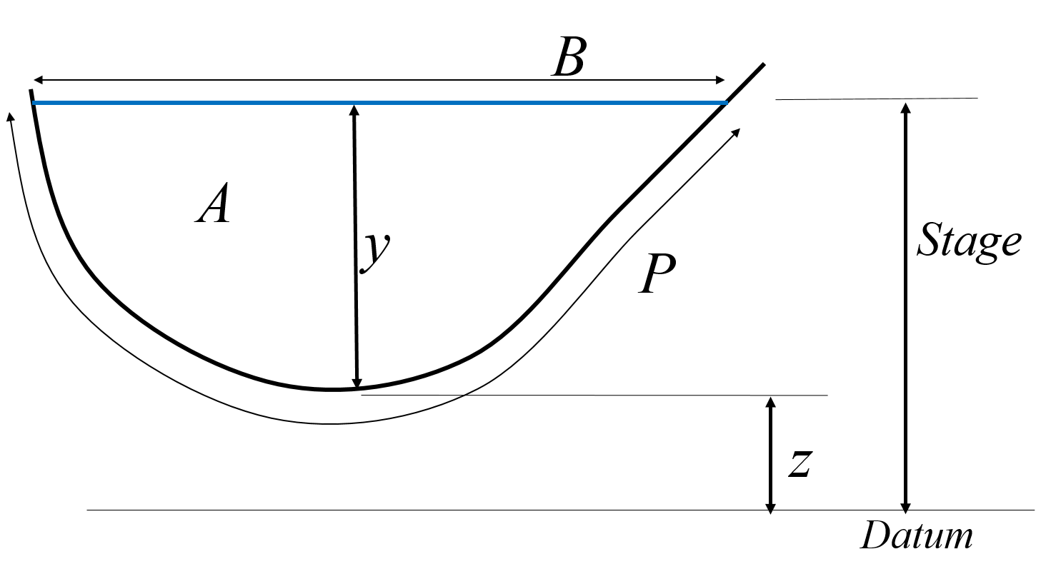
The commonly needed geometric properties are shown in figure 1.3 and defined as:

•

Depth ( $y$ ) - the vertical distance from the lowest point of the channel cross-section to the free surface.
•

Elevation ( $z$ ) - the vertical distance to a point in the channel (often the lowest point of the cross-section) from an arbitrary datum
•

Stage ( $WS$ ) - the vertical distance of the free surface from the same arbitrary datum that the Elevation is measured. (WS is short for Water Surface).
•

Area ( $A$ ) - the cross-sectional area of flow, normal to the direction of flow
•

Wetted perimeter ( $P$ ) - the length of the wetted surface measured normal to the direction of flow.
•

Surface width ( $B$ ) - width of the channel section at the free surface
•

Bed width ( $b$ ) - width of the channel section at the bed
•

Hydraulic radius ( $R$ ) - the ratio of area to wetted perimeter (A/P)
•

Hydraulic mean depth ( $D_{m}$ ) (or sometimes $\delta$ ) - the ratio of cross-sectional area to surface width $(A/B)$

[Uncaptioned image] — Table 1.2: Equations of Section Properties for Rectangular, Trapezoidal and Circular sections

1.4 Fundamental equations

The equations which describe the flow of fluid are derived from three fundamental laws of physics:

1.

Conservation of matter (or mass)
2.

Conservation of energy
3.

Conservation of momentum

Although first developed for solid bodies they are equally applicable to fluids. A brief description of the concepts is given below.

Conservation of matter
This says that matter can not be created nor destroyed, but it may be converted (e.g. by a chemical process.) In fluid mechanics, we do not consider chemical activity so the law reduces to one of conservation of mass.

Conservation of energy
This says that energy can not be created nor destroyed, but may be converted from one type to another (e.g. potential may be converted to kinetic energy). When engineers talk about energy "losses" they are referring to energy converted from mechanical (potential or kinetic) to some other form such as heat. A friction loss, for example, is a conversion of mechanical energy to heat. The basic equations can be obtained from the First Law of Thermodynamics but a simplified derivation will be given below.

Conservation of momentum
The law of conservation of momentum says that a moving body cannot gain or lose momentum unless acted upon by an external force. This is a statement of Newton’s Second Law of Motion:

\text{Force}=\text{rate of change of momentum}

In solid mechanics, these laws may be applied to an object which is has a fixed shape and is clearly defined. In fluid mechanics the object is not clearly defined and it may change shape constantly. To get over this we use the idea of control volumes. These are imaginary volumes of fluid within the body of the fluid. To derive the basic equation the above conservation laws are applied by considering the forces applied to the edges of a control volume within the fluid.

1.4.1 The Continuity Equation (conservation of mass)

For any control volume during the small time interval $\delta t$ the principle of conservation of mass implies that the mass of flow entering the control volume minus the mass of flow leaving the control volume equals the change of mass within.

If the flow is steady and the fluid incompressible the mass entering is equal to the mass leaving, so there is no change of mass within the control volume.

So for the time interval $\delta t$ :

\text{Mass flow entering}=\text{mass flow leaving}

Considering the control volume shown in Figure 1.4 which is a short length of open channel of arbitrary cross-section then, if $\rho$ is the fluid density and $Q$ is the volume flow rate then mass flow rate is $\rho Q$ and the continuity equation for steady incompressible flow can be written

\rho Q_{\text{entering}}=\rho Q_{\text{leaving}}

(1.1)

As, $Q$ , the volume flow rate is the product of the area and the mean velocity, then at the upstream face (face 1) where the mean velocity is $V_{1}$ and the cross-sectional area is $A_{1}$ then:

Similarly, at the downstream face, face 2, where mean velocity is $V_{2}$ and the cross-sectional area is $A_{2}$ then:

Q_{\text{leaving}}=V_{2}A_{2}

(1.2)

Therefore the continuity equation can be written as

V_{1}A_{1}=V_{2}A_{2}

(1.3)

1.4.2 The Energy equation (conservation of energy)

Consider the forms of energy available for the same control volume in Figure 1.4. If the fluid moves from the upstream face 1, to the downstream face 2 in time $\delta t$ over the length $L$ , then the work done in moving the fluid through face 1 during this time is

\text{work done}=\text{Force}\times\text{distance}=p_{1}A_{1}\times L

(1.4)

and the mass entering through face 1 is

\text{mass entering}=\text{density }\times\text{volume}=\rho_{1}\times A_{1}L

(1.5)

Therefore the kinetic energy of the system is:

\text{KE}=\frac{1}{2}mV^{2}_{1}=\frac{1}{2}\rho_{1}A_{1}LV_{1}^{2}

(1.6)

If $z_{1}$ is the height of the centroid of face 1, then the potential energy of the fluid entering the control volume is :

\text{PE}=mgz=\rho_{1}A_{1}Lgz_{1}

(1.7)

The total energy entering the control volume is the sum of the work done, the potential and the kinetic energy:

\text{Total Energy}=p_{1}A_{1}L+\frac{1}{2}\rho_{1}A_{1}LV_{1}^{2}+\rho_{1}A_{% 1}Lgz_{1}

(1.8)

We can write this in terms of energy per unit weight. As the weight of water entering the control volume is $\rho_{1}A_{1}Lg$ then just divide by this to get the total energy per unit weight:

\text{Total Energy per unit weight}=\frac{p_{1}}{\rho_{1}g}+\frac{V_{1}^{2}}{2% g}+z_{1}

(1.9)

At the exit to the control volume, face 2, similar considerations deduce

\text{Total Energy per unit weight}=\frac{p_{2}}{\rho_{2}g}+\frac{V_{2}^{2}}{2% g}+z_{2}

(1.10)

If no energy is supplied to the control volume from between the inlet and the outlet then energy leaving = energy entering and if the fluid is incompressible $\rho_{1}=\rho_{2}=\rho$

So,

At the exit to the control volume, face 2, similar considerations deduce

\frac{p_{1}}{\rho_{1}g}+\frac{V_{1}^{2}}{2g}+z_{1}=\frac{p_{2}}{\rho_{2}g}+% \frac{V_{2}^{2}}{2g}+z_{2}=H=\text{constant}

(1.11)

This is the Bernoulli equation.

Note:

1.

In the derivation of the Bernoulli equation it was assumed that no energy is lost in the control volume - i.e. the fluid is frictionless. To apply to non frictionless situations some energy loss terms must be included
2.

Each term in equation 1.11 has the dimensions of length (units of meters). For this reason, each term is often regarded as a "head" and given the names

$\begin{aligned} \frac{p}{\rho g}&=\text{pressure head}\\ \frac{V^{2}}{2g}&=\text{velocity head}\end{aligned}\qquad\qquad\begin{aligned}% z&=\text{potential head}\\ H&=\text{Total head}\end{aligned}$
3.

Although we derived the Bernoulli equation between two sections it should strictly speaking be applied along a streamline as the velocity will differ from the top to the bottom of the section. However, in engineering practice it is possible to apply the Bernoulli equation without reference to the particular streamline

Note: We can write $p=\rho gy$ so the term $\frac{p}{\rho g}=\frac{\rho gy}{\rho g}=y$ which results in the Bernoulli equation being written:

y_{1}+\frac{V_{1}^{2}}{2g}+z_{1}=y_{2}+\frac{V_{2}^{2}}{2g}+z_{2}=H=\text{constant}

We will see more on this later.

1.4.3 The momentum equation (momentum principle)

Again consider the control volume in Figure 1.4 during the small time period $\delta t$

	momentum entering	$\displaystyle=\rho\delta Q_{1}\>\delta t\>V_{1}$
	momentum leaving	$\displaystyle=\rho\delta Q_{2}\;\delta t\;V_{2}$

By the continuity principle : $\delta Q_{1}=\delta Q_{2}=\delta Q$ , and by applying Newton’s second law; Force = rate of change of momentum, we can write

	$\displaystyle\delta F$	$\displaystyle=\frac{\text{momentum leaving - momentum entering}}{\delta t}$
		$\displaystyle=\rho\>\delta Q(V_{2}-V_{1})$		(1.12)

It is more convenient to write the force on a control volume in each of the three, $x$ , $y$ and $z$ directions e.g. in the $x$ -direction

\delta F_{x}=\rho\>\delta Q(V_{2x}-V_{1x})

(1.13)

Integration over a volume gives the total force in the $x$ -direction as

F_{x}=\rho\>Q(V_{2x}-V_{1x})

(1.14)

We will usually drop the $x$ subscript when we describe one-dimensional flow in the $x$ -direction, to give

F=\rho\>Q(V_{2}-V_{1})

This is valid as long as velocity V is uniform over the whole cross-section.

This is the momentum equation for steady flow for a region of uniform velocity.

1.4.4 Energy and Momentum coefficients

In deriving the above momentum and energy (Bernoulli) equations it was noted that the velocity must be constant (equal to V) over the whole cross-section or constant along a stream-line. Clearly, this will not occur in practice. Fortunately, both these equations may still be used even for situations of quite non-uniform velocity distribution over a section. This is possible by the introduction of coefficients of energy and momentum, $\alpha$ and $\beta$ respectively.

These are defined as:

\alpha=\frac{\int\rho u^{3}\;dA}{\rho V^{3}A}

(1.15)

\beta=\frac{\int\rho u^{2}\;dA}{\rho V^{2}A}

(1.16)

where $V\;(=Q/A)$ is the mean velocity.

And the Bernoulli equation, Eqn 1.11, can be rewritten in terms of this mean velocity:

\frac{p}{\rho g}+\frac{\alpha V^{2}}{2g}+z=H=\text{constant}

(1.17)

And the general momentum equation becomes:

F=\rho\>Q\;\beta(V_{2}-V_{1})

(1.18)

The values of $\alpha$ and $\beta$ must be derived from the velocity distributions across a cross-section. They will always be greater than 1, but only by a small amount consequently, they can often be confidently omitted (i.e. set equal to 1) - but not always and their existence should always be remembered. For turbulent flow in a regular channel $\alpha$ does not usually go above 1.15 and $\beta$ will normally be below 1.05. We will see an example later where their inclusion is necessary to obtain accurate results.

1.5 Velocity distribution in open channels

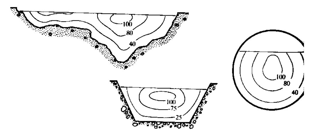
The measured velocity in an open channel will always vary across the channel section because of friction along the boundary. Adding to the complexity, this velocity distribution is not usually axisymmetric (as it is in pipe flow) due to the existence of the free surface. It might be expected to find the maximum velocity at the free surface where the shear force is zero but this is not the case. The maximum velocity is usually found just below the surface. The explanation for this is the presence of secondary currents which are circulating from the boundaries forwards the section centre. These have been found in both laboratory measurements and 3-dimensional numerical simulations of turbulence.

Figure 1.5 shows some typical velocity distributions across some channel cross-sections. The number indicates the percentage of maximum velocity.

1.5.1 Determination of energy and momentum coefficients

To determine the values of $\alpha$ and $\beta$ the velocity distribution must have been measured (or be known in some way). In irregular channels where the flow may be divided into distinct regions $\alpha$ may exceed 2 and should be included in the Bernoulli equation.

The figure below is a typical example of this situation. The channel may be of this shape when a river is in flood - this is known as a compound channel.

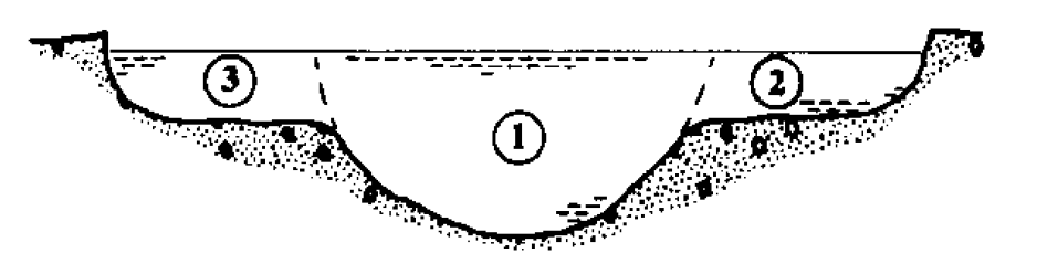
If the channel is divided as shown into three regions and making the assumption that $\alpha=1$ for each region (and assuming that $\rho$ is constant) then

\alpha=\frac{\int u^{3}\;dA}{\overline{V}^{3}\;A}=\frac{V_{1}^{3}A_{1}+V_{2}^{% 3}A_{2}+V_{3}^{3}A_{3}}{\overline{V}^{3}(A_{1}+A_{2}+A_{3})}

(1.19)

and similarly for $\beta$

\beta=\frac{\int u^{2}\;dA}{V^{2}A}=\frac{V_{1}^{2}A_{1}+V_{2}^{2}A_{2}+V_{3}^% {2}A_{3}}{\overline{V}^{2}(A_{1}+A_{2}+A_{3})}

(1.20)

where

\overline{V}=\frac{Q}{A}=\frac{V_{1}A_{1}+V_{2}A_{2}+V_{3}A_{3}}{A_{1}+A_{2}+A% _{3}}

(1.21)

1.6 Laminar and Turbulent flow

As in pipes, (and in all fluid flow), flow in an open channel may be either laminar or turbulent. The criterion for determining which is the Reynolds Number, $R_{e}$ .

For pipe flow (where $D$ is pipe diameter)

R_{e}=\frac{\rho VD}{\mu}=\frac{VD}{\nu}

(1.22)

And the limits for each type of flow are

	Laminar	$\displaystyle:R_{e\text{ pipe}}<2000$
	Turbulent	$\displaystyle:R_{e\text{ channel}}>4000$

If we take the characteristic length as the hydraulic radius $R=A/P$ then for a pipe just flowing full (i.e. not pressurised)

R=\frac{\pi D^{2}/4}{\pi D}=\frac{D}{4}

and

R_{e}=\frac{\rho VR}{\mu}=\frac{\rho V}{\mu}\frac{D}{4}=\frac{R_{e\text{ pipe}% }}{4}

(1.23)

So for an open channel, the limits for each type of flow become

	Laminar	$\displaystyle:R_{e\text{ channel}}<500$
	Turbulent	$\displaystyle:R_{e\text{ channel}}>1000$

In practice, the limit for turbulent flow is not so well defined in channel as it is in pipes and so 2000 is often taken as the threshold for turbulent flow.

1.7 Friction

We can draw further from pipe flow analysis to look at the effect of friction. Taking the Darcy-Wiesbach formula for head loss due to friction in a pipe in turbulent flow

h_{f}=\frac{4fLV^{2}}{2gD}

(1.24)

and make the substitution for hydraulic radius $R=D/4$ ,

S_{o}=\frac{fV^{2}}{2g\;R}

(1.25)

In uniform flow we can make the statement that the head loff due to friction $h_{f}$ divided by the length $L$ is equal to the slope of the channel, i.e.

S_{o}=\frac{h_{f}}{L}

(1.26)

and the friction coefficient $f$ can then be written

f=\frac{2gRS_{o}}{V^{2}}

(1.27)

As $\lambda=4f$ then we can also write

\lambda=\frac{8gRS_{o}}{V^{2}}

(1.28)

The Colebrook-White equation gives the $f-R_{e}$ , or $\lambda-R_{e}$ , relationship for pipes, putting in $R=D/4$ the pipe expressions gives and equivalent equation for open channels:

\frac{1}{\sqrt{f}}=-4\log_{10}\left(\frac{k_{s}}{14.8R}+\frac{1.26}{R_{e}\sqrt% {f}}\right)

(1.29)

which can be written for the $\lambda-R_{e}$ relationship as

\frac{1}{\sqrt{\lambda}}=-2\log_{10}\left(\frac{k_{s}}{3.7R}+\frac{2.51}{R_{e}% \sqrt{\lambda}}\right)

(1.30)

where $k_{s}$ is the effective roughness height.

A chart of the $\lambda-R_{e}$ relationship for open channels can be drawn using this equation but its practical application is not as clear as for pipes. In pipes this relationship is useful but due to the more complex flow pattern and the extra variable (as hydraulic radius, $R$ , varies with depth and channel shape) then it is difficult to apply to a particular channel. The general approach is also questionable as there has been no account taken for a free surface which changes velocity distributions considerably causing frictional resistance to be much less uniform in open channels than in pipes.

In practice flow in open channels is usually in the rough turbulent zone and consequently simpler friction formulae may be applied to relate frictional losses to velocity and channel shape.

1.8 The Froude number

The Froude number is an important number in open channel flow and is defined as:

F_{r}=\frac{V}{\sqrt{gD_{m}}}

(1.31)

Its physical significance is the ratio of inertial forces to gravitational forces squared

F_{r}^{2}=\frac{\text{inertial force}}{\text{gravitational force}}

It can also be interpreted as the ratio of water velocity to wave velocity

F_{r}=\frac{\text{water velocity}}{\text{wave velocity}}

This is an extremely useful non-dimensional number in open-channel hydraulics.

Although these terms will be defined later, it is useful to state them here: the value of $F_{r}$ determines the regime of flow - sub, super or critical (see later), and the direction in which disturbances travel. These may be summarised as:

$F_{r}<1$	sub-critical
	water velocity $<$ wave velocity
	upstream levels are affected by downstream levels
$F_{r}=1$	critical
$F_{r}>1$	super-critical
	water velocity $>$ wave velocity
	upstream levels are NOT affected by downstream levels

We will later be interested in the depth at which critical flow occurs i.e. the depth when $F_{r}=1$ which is know as critical depth, $y_{c}$ .

	Rectangle	Trapezoid	Circle

			( $\phi$ in radians)
Area, $A$	$by$	$(b+sy)y$	$\frac{1}{8}(\phi-\sin\phi)D^{2}$
Wetted perimeter, $P$	$b+2y$	$b+2y\sqrt{1+s^{2}}$	$\frac{1}{2}\phi D$
Top width, $B$	$b$	$b+2sy$	$(\sin(\phi/2))D$
Hydraulic Radius, $R=\frac{A}{P}$	$\frac{by}{b+2y}$	$\frac{(b+sy)y}{b+2y\sqrt{1+s^{2}}}$	$\frac{1}{4}\left(1-\frac{\sin\phi}{\phi}\right)D$
Hydraulic mean depth, $D_{m}=\frac{A}{B}$	$y$	$\frac{(b+sy)y}{b+2sy}$	$\frac{1}{8}\left(\frac{\phi-\sin\phi}{\sin(\phi/2)}\right)D$