5 How Fluid Flow is Affected by Boundaries ‣ CIVE1460: Properties of Materials: Water, Soil, Steel and Timber An Introduction to Engineering Fluids Mechanics Water Engineering I‣ CIVE1460: Properties of Materials: Water, Soil, Steel and Timber An Introduction to Engineering Fluids Mechanics Water Engineering I

5.1 Real fluids

The flow of real fluids exhibits viscous effect, that is they tend to ”stick” to solid surfaces and have stresses within their body.

You might remember from earlier in the course Newtons law of viscosity:

\tau\propto\frac{du}{dy}

This tells us that the shear stress, $\tau$ , in a fluid is proportional to the velocity velocity gradient - the rate of change of velocity across the fluid path. For a ”Newtonian” fluid we can write:

\tau=\mu\frac{du}{dy}

where the constant of proportionality, $\mu$ is known as the coefficient of viscosity (or simply viscosity). We saw that for some fluids - sometimes known as exotic fluids, or non-Newtonian fluids where the value of $\mu$ changes with stress or velocity gradient. We shall only deal with Newtonian fluids.

In his lecture we shall look at how the forces due to momentum changes on the fluid and viscous forces compare and what changes take place.

5.2 Laminar and turbulent flow

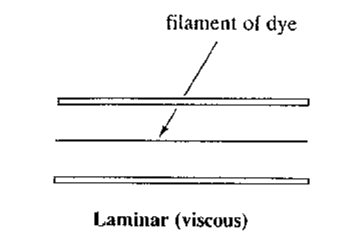
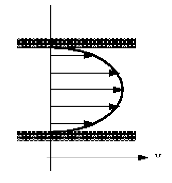
If we were to take a pipe of free flowing water and inject a dye into the middle of the stream, what would we expect to happen?

This

this

or this

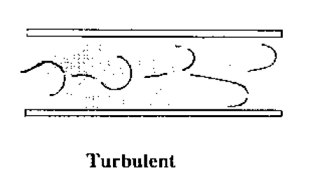
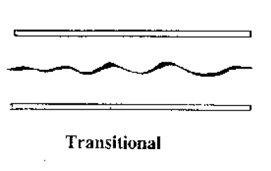
Actually both would happen - but for different flow rates. The top occurs when the fluid is flowing fast and the lower when it is flowing slowly.

The top situation is known as turbulent flow and the lower as laminar flow. In laminar flow the motion of the particles of fluid is very orderly with all particles moving in straight lines parallel to the pipe walls.

But what is fast or slow? And at what speed does the flow pattern change? And why might we want to know this?

The phenomenon was first investigated in the 1880s by Osbourne Reynolds in an experiment which has become a classic in fluid mechanics.

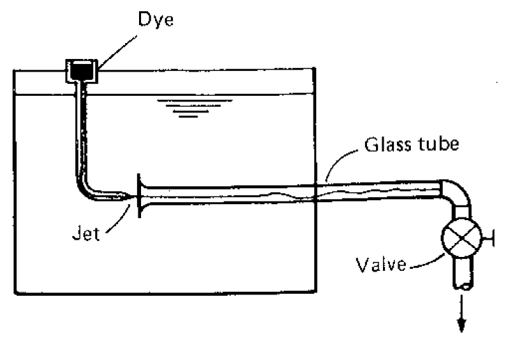
He used a tank arranged as above with a pipe taking water from the centre into which he injected a dye through a needle. After many experiments he saw that this expression

\frac{\rho ud}{\mu}

where $\rho$ = density, $u$ = mean velocity, $d$ = diameter and $\mu$ = viscosity

would help predict the change in flow type. If the value is less than about 2000 then flow is laminar, if greater than 4000 then turbulent and in between these then in the transition zone.

This value is known as the Reynolds number, $Re$ :

Laminar flow:			$Re$	$<$	2000
Transitional flow:	2000	$<$	$Re$	$<$	4000
Turbulent flow:			$Re$	$>$	4000

What are the units of this Reynolds number? We can fill in the equation with SI units:

\rho=kg/m^{3},\qquad u=m/s,\qquad d=m\\ \mu=Ns/m^{2}=kg/ms

Re=\frac{\rho ud}{\mu}\qquad\text{in terms of units: }\equiv\frac{kg}{m^{3}}% \frac{m}{s}\frac{m}{1}\frac{ms}{kg}\equiv 1

i.e. $Re$ has no units. A quantity that has no units is known as a non-dimensional (or dimensionless) quantity. Thus the Reynolds number, $Re$ , is a non-dimensional number.

We can go through an example to discover at what velocity the flow in a pipe stops being laminar. If the pipe and the fluid have the following properties:

Water density	$\rho=1000\;kg/m^{3}$
Pipe diameter	$d=0.5\;m$
(dynamic) viscosity	$\mu=0.55^{-3}\;Ns/m^{2}$

We want to know the maximum velocity when the $Re$ is 2000.

	$\displaystyle Re$	$\displaystyle=\frac{\rho ud}{\mu}=2000$
	$\displaystyle u$	$\displaystyle=\frac{2000\mu}{\rho d}=\frac{2000\times 0.55^{-3}}{1000\times 0.5}$
	$\displaystyle u$	$\displaystyle=0.0022\;m/s=2.2\;mm/s$

If this were a pipe in a house central heating system, where the pipe diameter is typically $0.015\;m$ , the limiting velocity for laminar flow would be, $0.0733\;m/s$ .

Both of these are very slow. In practice it very rarely occurs in a piped water system - the velocities of flow are much greater. Laminar flow does occur in situations with fluids of greater viscosity - e.g. in bearing with oil as the lubricant.

At small values of $Re$ above 2000 the flow exhibits small instabilities. At values of about 4000 we can say that the flow is truly turbulent. Over the past 100 years since this experiment, numerous more experiments have shown this phenomenon of limits of $Re$ for many different Newtonian fluids - including gasses.

What does this abstract number mean?

We can say that the number has a physical meaning, by doing so it helps to understand some of the reasons for the changes from laminar to turbulent flow.

	$\displaystyle Re$	$\displaystyle=\frac{\rho ud}{\mu}$
		$\displaystyle\frac{\text{inertial forces}}{\text{viscous forces}}$

It can be interpreted that when the inertial forces dominate over the viscous forces (when the fluid is flowing faster and $Re$ is larger) then the flow is turbulent. When the viscous forces are dominant (slow flow, low Re) they are sufficient enough to keep all the fluid particles in line, then the flow is laminar.

In summary:

Laminar flow

•

$Re<2000$
•

’low’ velocity
•

Dye does not mix with water
•

Fluid particles move in straight lines
•

Simple mathematical analysis possible
•

Rare in practice in water systems.

Transitional flow

•

$2000>Re<4000$
•

’medium’ velocity
•

Dye stream wavers in water - mixes slightly.

Turbulent flow

•

$Re>4000$
•

’high’ velocity
•

Dye mixes rapidly and completely
•

Particle paths completely irregular
•

Average motion is in the direction of the flow
•

Cannot be seen by the naked eye
•

Changes/fluctuations are very difficult to detect. Must use laser.
•

Mathematical analysis very difficult - so experimental measures are used
•

Most common type of flow.

5.3 Pressure loss due to friction in a pipeline.

Up to this point on the course we have considered ideal fluids where there have been no losses due to friction or any other factors. In reality, because fluids are viscous, energy is lost by flowing fluids due to friction which must be taken into account. The effect of the friction shows itself as a pressure (or head) loss.

In a pipe with a real fluid flowing, at the wall there is a shearing stress retarding the flow, as shown below.

If a manometer is attached as the pressure (head) difference due to the energy lost by the fluid overcoming the shear stress can be easily seen.

The pressure at 1 (upstream) is higher than the pressure at 2.

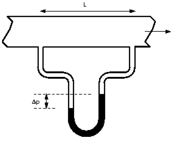
We can do some analysis to express this loss in pressure in terms of the forces acting on the fluid. Consider a cylindrical element of incompressible fluid flowing in the pipe, as shown

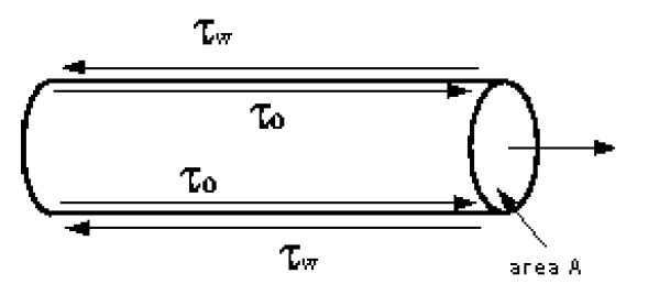
The pressure at the upstream end is $p$ , and at the downstream end the pressure has fallen by $\Delta p$ to $(p-\Delta p)$ .

The driving force due to pressure ( $F=\text{Pressure}x\text{Area}$ ) can then be written

	driving force	$\displaystyle=\text{Pressure force at 1}-\text{Pressure force at 2}$
		$\displaystyle=pA-\left(p-\Delta p\right)$
		$\displaystyle=\Delta p\;A$
		$\displaystyle=\Delta p\frac{\pi d^{2}}{4}$

The retarding force is that due to the shear stress by the walls

	retarding force	$\displaystyle=\text{shear stress}\times\text{area over which it acts}$
		$\displaystyle=\tau_{w}\times\text{area of the pipe wall}$
		$\displaystyle=\tau_{w}\pi dL$

As the flow is in equilibrium,

	driving force	$\displaystyle=\text{retarding force}$
	$\displaystyle\Delta p\frac{\pi d^{2}}{4}$	$\displaystyle=\tau_{w}\pi dL$
	$\displaystyle\Delta p$	$\displaystyle=\frac{\tau_{w}4L}{d}$

Giving an expression for pressure loss in a pipe in terms of the pipe diameter and the shear stress at the wall on the pipe.

The shear stress will vary with velocity of flow and hence with $Re$ . Many experiments have been done with various fluids measuring the pressure loss at various Reynolds numbers. These results plotted to show a graph of the relationship between pressure loss and Re look similar to the figure below:

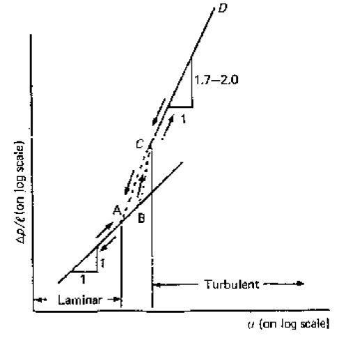
This graph shows that the relationship between pressure loss and $Re$ can be expressed as

laminar	$\Delta p\propto u$
turbulent	$\Delta p\propto u^{1.7\text{ (to 2.0)}}$

As these are empirical relationships, they help in determining the pressure loss but not in finding the magnitude of the shear stress at the wall ?w on a particular fluid. If we knew ?w we could then use it to give a general equation to predict the pressure loss.

5.4 Pressure loss during laminar flow in a pipe

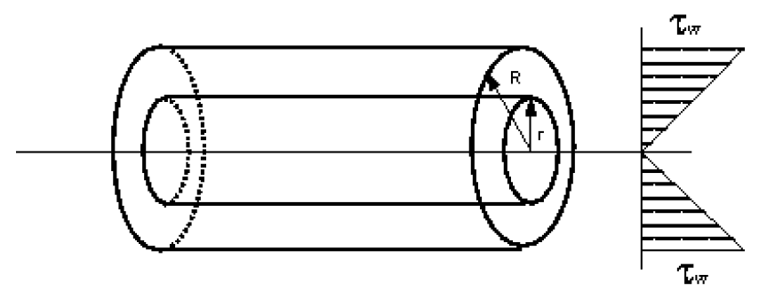
In general the shear stress $\tau_{w}$ . is almost impossible to measure. But for laminar flow it is possible to calculate a theoretical value for a given velocity, fluid and pipe dimension.

In laminar flow the paths of individual particles of fluid do not cross, so the flow may be considered as a series of concentric cylinders sliding over each other - rather like the cylinders of a collapsible pocket telescope.

As before, consider a cylinder of fluid, length $L$ , radius $r$ , flowing steadily in the centre of a pipe.

We are in equilibrium, so the shearing forces on the cylinder equal the pressure forces.

	$\displaystyle\tau 2\pi rL$	$\displaystyle=\Delta pA=\Delta p\pi R^{2}$
	$\displaystyle\tau$	$\displaystyle=\frac{\Delta p}{L}\frac{r}{2}$

By Newtons law of viscosity we have $\tau=\mu\frac{du}{dy}$ , where $y$ is the distance from the wall. As we are measuring from the pipe centre then we change the sign and replace $y$ with $r$ , the distance from the centre, giving

\tau=-\mu\frac{du}{dr}

Which can be combined with the equation above to give

	$\displaystyle\frac{\Delta p}{L}\frac{r}{2}$	$\displaystyle=-\mu\frac{du}{dr}$
	$\displaystyle\frac{du}{dr}$	$\displaystyle=-\frac{\Delta p}{L}\frac{r}{2\mu}$

In an integral form this gives an expression for velocity,

u=-\frac{\Delta p}{L}\frac{1}{2\mu}\int r\;dr

Integrating gives the value of velocity at a point distance r from the centre

u_{r}=-\frac{\Delta p}{L}\frac{r^{2}}{4\mu}+C

At $r=0$ , (the centre of the pipe), $u=u_{max}$ , at $r=R$ (the pipe wall) $u=0$ , giving

C=\frac{\Delta p}{L}\frac{R^{2}}{4\mu}

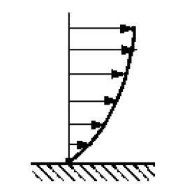
so, an expression for velocity at a point r from the pipe centre when the flow is laminar is

u_{r}=\frac{\Delta p}{L}\frac{1}{4\mu}\left(R^{2}-r^{2}\right)

Note how this is a parabolic profile (of the form $y=ax^{2}+b$ ) so the velocity profile in the pipe looks similar to the figure below

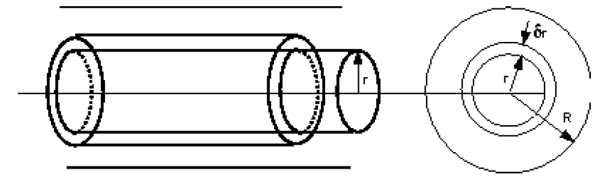
What is the discharge in the pipe?

	$\displaystyle Q$	$\displaystyle=u_{m}A$
	$\displaystyle u_{m}$	$\displaystyle=\int_{0}^{R}u_{r}\;dr$
		$\displaystyle=\frac{\Delta p}{L}\frac{1}{4\mu}\int_{0}^{R}\left(R^{2}-r^{2}% \right)\;dr$
		$\displaystyle=\frac{\Delta p}{L}\frac{R^{2}}{8\mu}$
		$\displaystyle=\frac{\Delta pd^{2}}{32\mu L}$

So the discharge can be written

	$\displaystyle Q$	$\displaystyle=\frac{\Delta pd^{2}}{32\mu L}\frac{\pi d^{2}}{4}$
		$\displaystyle=\frac{\Delta p}{L}\frac{\pi d^{2}}{128\mu L}$

This is the Hagen-Poiseuille equation for laminar flow in a pipe. It expresses the discharge $Q$ in terms of the pressure gradient ( $\frac{\delta p}{\delta x}=\frac{\Delta p}{dL}$ ), diameter of the pipe and the viscosity of the fluid.

We are interested in the pressure loss (head loss) and want to relate this to the velocity of the flow. Writing pressure loss in terms of head loss $h_{f}$ , i.e. $p=\rho gh_{f}$ :

u=\frac{\rho gh_{f}d^{2}}{32\mu L}

h_{f}=\frac{32\mu Lu}{\rho gd^{2}}

This shows that pressure loss is directly proportional to the velocity when flow is laminar.

It has been validated many time by experiment.

It justifies two assumptions:

1.

fluid does not slip past a solid boundary
2.

Newtons hypothesis.

5.5 Boundary Layers

(Recommended extra reading for this section: Fluid Mechanics by Douglas J F, Gasiorek J M, and Swaffield J A. Longman publishers. Pages 327-332.)

When a fluid flows over a stationary surface, e.g. the bed of a river, or the wall of a pipe, the fluid touching the surface is brought to rest by the shear stress ?o at the wall. The velocity increases from the wall to a maximum in the main stream of the flow.

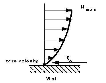
Looking at this two-dimensionally we get the above velocity profile from the wall to the centre of the flow.

This profile doesn’t just exit, it must build up gradually from the point where the fluid starts to flow past the surface - e.g. when it enters a pipe.

If we consider a flat plate in the middle of a fluid, we will look at the build up of the velocity profile as the fluid moves over the plate.

Upstream the velocity profile is uniform, (free stream flow) a long way downstream we have the velocity profile we have talked about above. This is the known as fully developed flow. But how do we get to that state?

This region, where there is a velocity profile in the flow due to the shear stress at the wall, we call the boundary layer. The stages of the formation of the boundary layer are shown in the figure below:

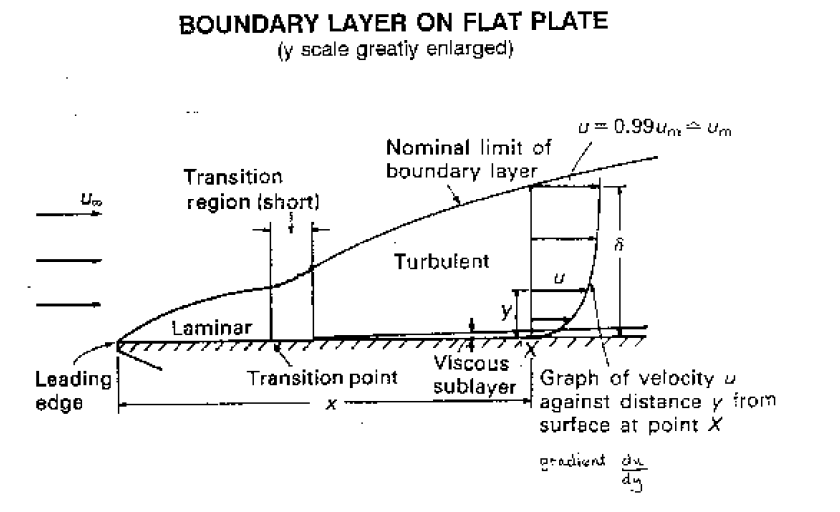
We define the thickness of this boundary layer as the distance from the wall to the point where the velocity is 99% of the free stream velocity, the velocity in the middle of the pipe or river.

\text{boundary layer thickness,}\delta=\text{distance from wall to point where% }u=0.99u_{\text{mainstream}}

The value of $\delta$ will increase with distance from the point where the fluid first starts to pass over the boundary - the flat plate in our example. It increases to a maximum in fully developed flow.

Correspondingly, the drag force $D$ on the fluid due to shear stress $\tau_{o}$ at the wall increases from zero at the start of the plate to a maximum in the fully developed flow region where it remains constant. We can calculate the magnitude of the drag force by using the momentum equation. But this complex and not necessary for this course.

Our interest in the boundary layer is that its presence greatly affects the flow through or round an object. So here we will examine some of the phenomena associated with the boundary layer and discuss why these occur.

5.6 Formation of the boundary layer

Above we noted that the boundary layer grows from zero when a fluid starts to flow over a solid surface. As is passes over a greater length more fluid is slowed by friction between the fluid layers close to the boundary. Hence the thickness of the slower layer increases. The fluid near the top of the boundary layer is dragging the fluid nearer to the solid surface along. The mechanism for this dragging may be one of two types:

The first type occurs when the normal viscous forces (the forces which hold the fluid together) are large enough to exert drag effects on the slower moving fluid close to the solid boundary. If the boundary layer is thin then the velocity gradient normal to the surface, ( $du/dy$ ), is large so by Newton’s law of viscosity the shear stress, $\tau=\mu(du/dy)$ , is also large. The corresponding force may then be large enough to exert drag on the fluid close to the surface.

As the boundary layer thickness becomes greater, so the velocity gradient become smaller and the shear stress decreases until it is no longer enough to drag the slow fluid near the surface along. If this viscous force was the only action then the fluid would come to a rest.

It, of course, does not come to rest but the second mechanism comes into play. Up to this point the flow has been laminar and Newton’s law of viscosity has applied. This part of the boundary layer is known as the laminar boundary layer.

The viscous shear stresses have held the fluid particles in a constant motion within layers. They become small as the boundary layer increases in thickness and the velocity gradient gets smaller. Eventually they are no longer able to hold the flow in layers and the fluid starts to rotate.

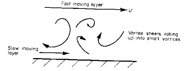
This causes the fluid motion to rapidly becomes turbulent. Fluid from the fast moving region moves to the slower zone transferring momentum and thus maintaining the fluid by the wall in motion. Conversely, slow moving fluid moves to the faster moving region slowing it down. The net effect is an increase in momentum in the boundary layer. We call the part of the boundary layer the turbulent boundary layer.

At points very close to the boundary the velocity gradients become very large and the velocity gradients become very large with the viscous shear forces again becoming large enough to maintain the fluid in laminar motion. This region is known as the laminar sub-layer. This layer occurs within the turbulent zone and is next to the wall and very thin - a few hundredths of a $mm$ .

Surface roughness effect

Despite its thinness, the laminar sub-layer can play a vital role in the friction characteristics of the surface.

This is particularly relevant when defining pipe friction - as will be seen in more detail in the level 2 module. In turbulent flow if the height of the roughness of a pipe is greater than the thickness of the laminar sub-layer then this increases the amount of turbulence and energy losses in the flow. If the height of roughness is less than the thickness of the laminar sub-layer the pipe is said to be smooth and it has little effect on the boundary layer.

In laminar flow the height of roughness has very little effect

5.7 Boundary layers in pipes

As flow enters a pipe the boundary layer will initially be of the laminar form. This will change depending on the ration of inertial and viscous forces; i.e. whether we have laminar (viscous forces high) or turbulent flow (inertial forces high).

From earlier we saw how we could calculate whether a particular flow in a pipe is laminar or turbulent using the Reynolds number.

Re=\frac{\rho ud}{\mu}

$\rho=$ density, $u=$ velocity $\mu=$ viscosity $d=$ pipe diameter)

Laminar flow:			$Re$	$<$	2000
Transitional flow:	2000	$<$	$Re$	$<$	4000
Turbulent flow:			$Re$	$>$	4000

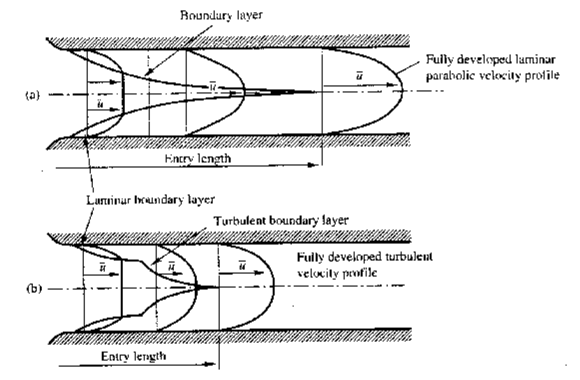
If we only have laminar flow the profile is parabolic - as proved in earlier lectures - as only the first part of the boundary layer growth diagram is used. So we get the top diagram in the above figure.

If turbulent (or transitional), both the laminar and the turbulent (transitional) zones of the boundary layer growth diagram are used. The growth of the velocity profile is thus like the bottom diagram in the above figure.

Once the boundary layer has reached the centre of the pipe the flow is said to be fully developed. (Note that at this point the whole of the fluid is now affected by the boundary friction.)

The length of pipe before fully developed flow is achieved is different for the two types of flow. The length is known as the entry length.

Laminar flow entry length:	$\approx 120\times$ diameter
Transitional flow:	$\approx 60\times$ diameter

5.8 Boundary layer separation

5.9 Convergent flows: Negative pressure gradients

If flow over a boundary occurs when there is a pressure decrease in the direction of flow, the fluid will accelerate and the boundary layer will become thinner. This is the case for convergent flows.

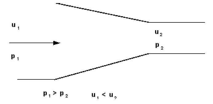
The accelerating fluid maintains the fluid close to the wall in motion. Hence the flow remains stable and turbulence reduces. Boundary layer separation does not occur.

5.10 Divergent flows: Positive pressure gradients

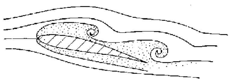
When the pressure increases in the direction of flow the situation is very different. Fluid outside the boundary layer has enough momentum to overcome this pressure which is trying to push it backwards. The fluid within the boundary layer has so little momentum that it will very quickly be brought to rest, and possibly reversed in direction. If this reversal occurs it lifts the boundary layer away from the surface as shown below.

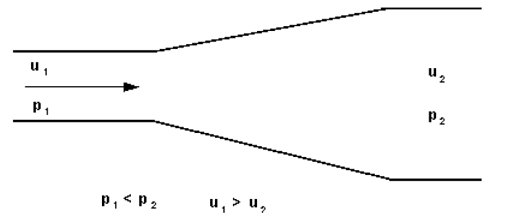
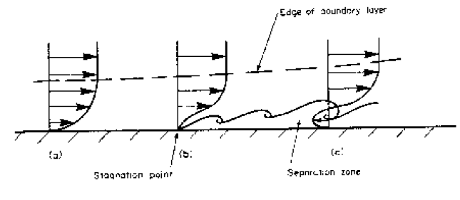
This phenomenon is known as boundary layer separation.

At the edge of the separated boundary layer, where the velocities change direction, a line of vortices occur (known as a vortex sheet). This happens because fluid to either side is moving in the opposite direction.

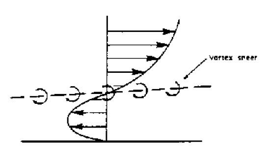
This boundary layer separation and increase in the turbulence because of the vortices results in very large energy losses in the flow.

These separating / divergent flows are inherently unstable and far more energy is lost than in parallel or convergent flow.

5.11 Examples of boundary layer separation

5.11.1 A divergent duct or diffuser

The increasing area of flow causes a velocity drop (according to continuity) and hence a pressure rise (according to the Bernoulli equation).

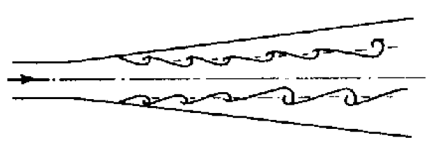
Increasing the angle of the diffuser increases the probability of boundary layer separation. In a Venturi meter it has been found that an angle of about $6^{o}$ provides the optimum balance between length of meter and danger of boundary layer separation which would cause unacceptable pressure energy losses.

5.11.2 Tee-Junctions

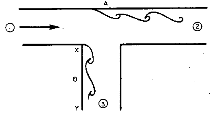
Assuming equal sized pipes, as fluid is removed, the velocities at 2 and 3 are smaller than at 1, the entrance to the tee. Thus the pressure at 2 and 3 are higher than at 1. These two adverse pressure gradients can cause the two separations shown in the diagram above.

5.11.3 Y-Junctions

Tee junctions are special cases of the Y-junction with similar separation zones occurring. See the diagram below.

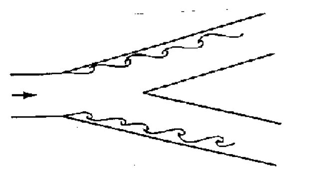
Downstream, away from the junction, the boundary layer reattaches and normal flow occurs i.e. the effect of the boundary layer separation is only local. Nevertheless fluid downstream of the junction will have lost energy.

5.11.4 Bends

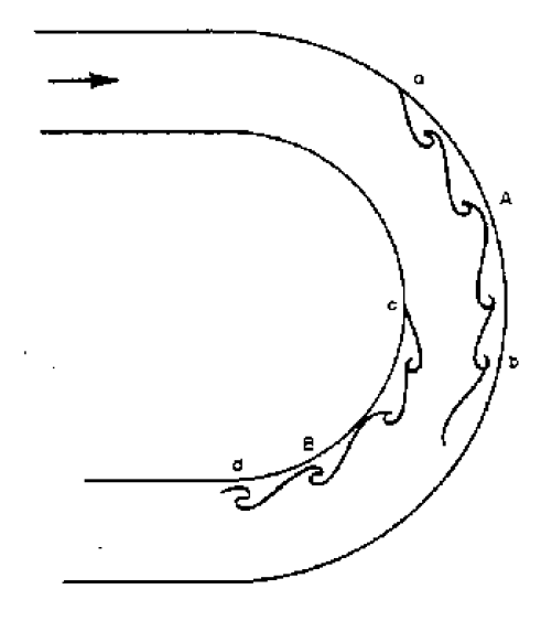
Two separation zones occur in bends as shown above. The pressure at b must be greater than at a as it must provide the required radial acceleration for the fluid to get round the bend. There is thus an adverse pressure gradient between a and b so separation may occur here.

Pressure at c is less than at the entrance to the bend but pressure at d has returned to near the entrance value - again this adverse pressure gradient may cause boundary layer separation.

5.11.5 Flow past a cylinder

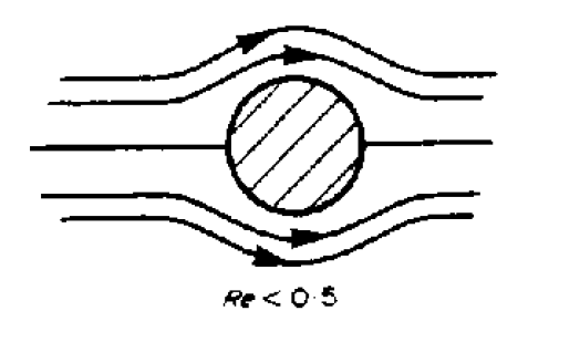
The pattern of flow around a cylinder varies with the velocity of flow. If flow is very slow with the Reynolds number (? v diameter/?? less than 0.5, then there is no separation of the boundary layers as the pressure difference around the cylinder is very small. The pattern is something like that in the figure below.

If $2<Re<70$ then the boundary layers separate symmetrically on either side of the cylinder. The ends of these separated zones remain attached to the cylinder, as shown below.

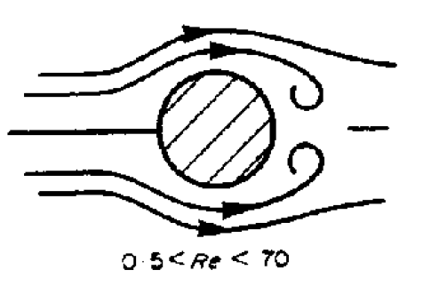
Above a $Re$ of 70 the ends of the separated zones curl up into vortices and detach alternately from each side forming a trail of vortices on the down stream side of the cylinder. This trial in known as a Karman vortex trail or street. This vortex trail can easily be seen in a river by looking over a bridge where there is a pier to see the line of vortices flowing away from the bridge. The phenomenon is responsible for the whistling of hanging telephone or power cables. A more significant event was the famous failure of the Tacoma narrows bridge. Here the frequency of the alternate vortex shedding matched the natural frequency of the bridge deck and resonance amplified the vibrations until the bridge collapsed. (The frequency of vortex shedding from a cylinder can be predicted. We will not try to predict it here but a derivation of the expression can be found in many fluid mechanics text books.)

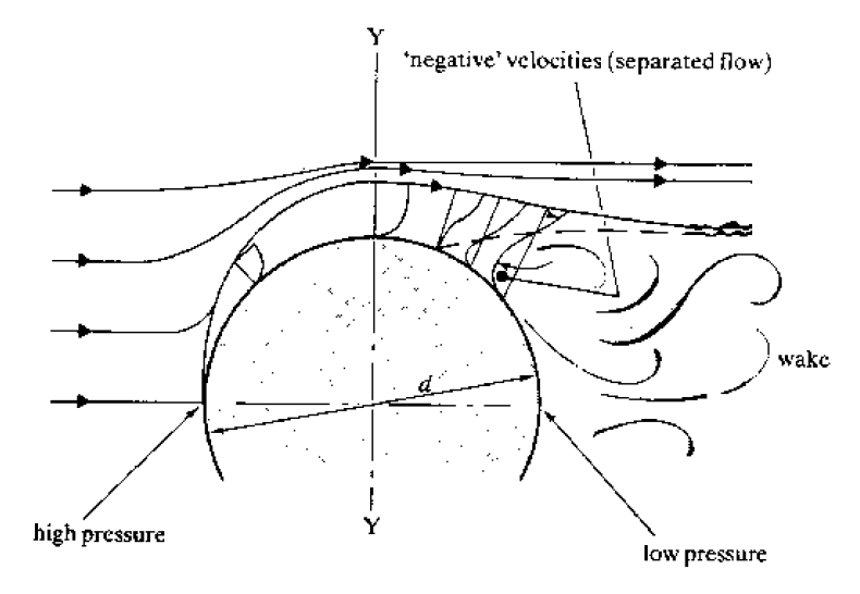
Looking at the figure above, the formation of the separation occurs as the fluid accelerates from the centre to get round the cylinder (it must accelerate as it has further to go than the surrounding fluid). It reaches a maximum at Y, where it also has also dropped in pressure. The adverse pressure gradient between here and the downstream side of the cylinder will cause the boundary layer separation if the flow is fast enough, ( $Re>200$ .)

5.11.6 Aerofoil

Normal flow over a aerofoil (a wing cross-section) is shown in the figure below with the boundary layers greatly exaggerated.

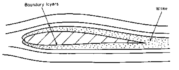
The velocity increases as air it flows over the wing. The pressure distribution is similar to that shown below so transverse lift force occurs.

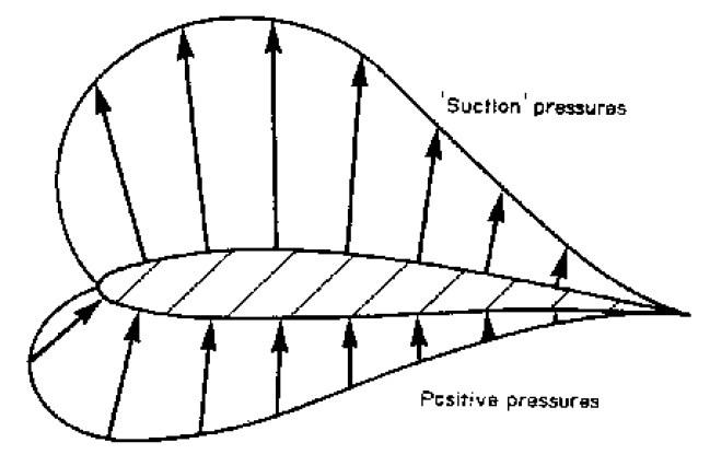
If the angle of the wing becomes too great and boundary layer separation occurs on the top of the aerofoil the pressure pattern will change dramatically. This phenomenon is known as stalling.

When stalling occurs, all, or most, of the ’suction’ pressure is lost, and the plane will suddenly drop from the sky! The only solution to this is to put the plane into a dive to regain the boundary layer. A transverse lift force is then exerted on the wing which gives the pilot some control and allows the plane to be pulled out of the dive.

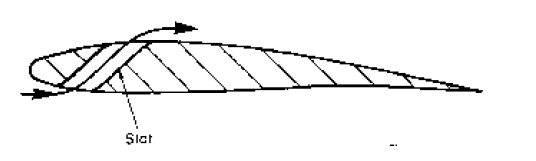
Fortunately there are some mechanisms for preventing stalling. They all rely on preventing the boundary layer from separating in the first place.

1.

Arranging the engine intakes so that they draw slow air from the boundary layer at the rear of the wing though small holes helps to keep the boundary layer close to the wing. Greater pressure gradients can be maintained before separation take place.
2.

Slower moving air on the upper surface can be increased in speed by bringing air from the high pressure area on the bottom of the wing through slots. Pressure will decrease on the top so the adverse pressure gradient which would cause the boundary layer separation reduces.

Figure 103: A slot to put fast moving flow over the top of the aerofoil
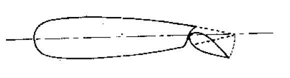
3.

Putting a flap on the end of the wing and tilting it before separation occurs increases the velocity over the top of the wing, again reducing the pressure and chance of separation occurring.

Figure 104: A flap on a aerofoil to change velocity and pressure profile over teh aerofoil