4 Fluid Dynamics ‣ CIVE1460: Properties of Materials: Water, Soil, Steel and Timber An Introduction to Engineering Fluids Mechanics Water Engineering I‣ CIVE1460: Properties of Materials: Water, Soil, Steel and Timber An Introduction to Engineering Fluids Mechanics Water Engineering I

4.1 Uniform Flow, Steady Flow

It is possible - and useful - to classify the type of flow which is being examined into small number of groups.

If we look at a fluid flowing under normal circumstances - a river for example - the conditions at one point will vary from those at another point (e.g. different velocity) we have non-uniform flow.

If the conditions at one point vary as time passes then we have unsteady flow.

Under some circumstances the flow will not be as changeable as this. He following terms describe the states which are used to classify fluid flow:

•

uniform flow: If the flow velocity is the same magnitude and direction at every point in the fluid it is said to be uniform.
•

non-uniform: If at a given instant, the velocity is not the same at every point the flow is non-uniform. (In practice, by this definition, every fluid that flows near a solid boundary will be non-uniform - as the fluid at the boundary must take the speed of the boundary, usually zero. However if the size and shape of the of the cross-section of the stream of fluid is constant the flow is considered uniform.)
•

steady: A steady flow is one in which the conditions (velocity, pressure and cross-section) may differ from point to point but DO NOT change with time.
•

unsteady: If at any point in the fluid, the conditions change with time, the flow is described as unsteady. (In practise there is always slight variations in velocity and pressure, but if the average values are constant, the flow is considered steady.

Combining the above we can classify any flow in to one of four type:

a

Steady uniform flow. Conditions do not change with position in the stream or with time. An example is the flow of water in a pipe of constant diameter at constant velocity.
b

Steady non-uniform flow. Conditions change from point to point in the stream but do not change with time. An example is flow in a tapering pipe with constant velocity at the inlet - velocity will change as you move along the length of the pipe toward the exit.
c

Unsteady uniform flow. At a given instant in time the conditions at every point are the same, but will change with time. An example is a pipe of constant diameter connected to a pump pumping at a constant rate which is then switched off.
d

Unsteady non-uniform flow. Every condition of the flow may change from point to point and with time at every point. For example waves in a channel.

If you imaging the flow in each of the above classes you may imagine that one class is more complex than another. And this is the case - steady uniform flow is by far the most simple of the four. You will then be pleased to hear that this course is restricted to only this class of flow. We will not be encountering any non-uniform or unsteady effects in any of the examples (except for one or two quasi-time dependent problems which can be treated at steady).

4.2 Compressible or Incompressible

All fluids are compressible - even water - their density will change as pressure changes. Under steady conditions, and provided that the changes in pressure are small, it is usually possible to simplify analysis of the flow by assuming it is incompressible and has constant density. As you will appreciate, liquids are quite difficult to compress - so under most steady conditions they are treated as incompressible. In some unsteady conditions very high pressure differences can occur and it is necessary to take these into account - even for liquids. Gasses, on the contrary, are very easily compressed, it is essential in most cases to treat these as compressible, taking changes in pressure into account.

4.3 Three-dimensional flow

Although in general all fluids flow three-dimensionally, with pressures and velocities and other flow properties varying in all directions, in many cases the greatest changes only occur in two directions or even only in one. In these cases changes in the other direction can be effectively ignored making analysis much more simple.

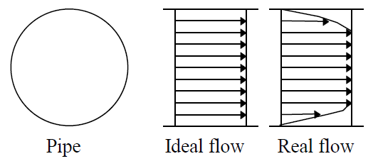
Flow is one dimensional if the flow parameters (such as velocity, pressure, depth etc.) at a given instant in time only vary in the direction of flow and not across the cross-section. The flow may be unsteady, in this case the parameter vary in time but still not across the cross-section. An example of one-dimensional flow is the flow in a pipe. Note that since flow must be zero at the pipe wall - yet non-zero in the centre - there is a difference of parameters across the cross-section. Should this be treated as two-dimensional flow? Possibly - but it is only necessary if very high accuracy is required. A correction factor is then usually applied.

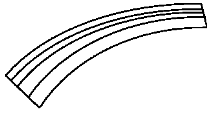
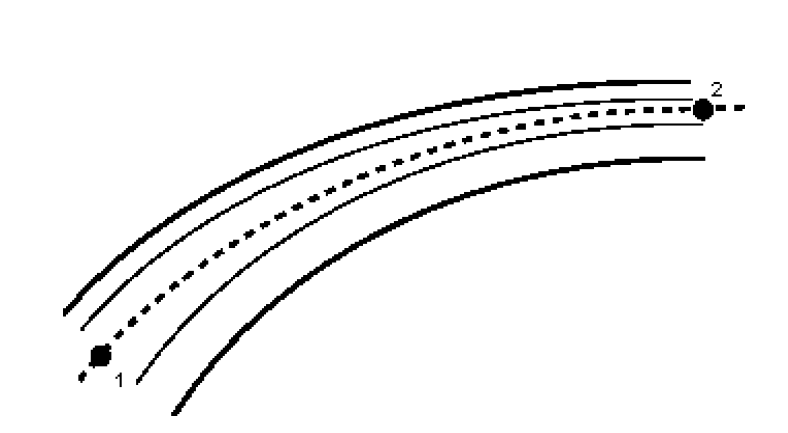
Refer to caption — Figure 27: One dimensional flow in a pipe.

Flow is two-dimensional if it can be assumed that the flow parameters vary in the direction of flow and in one direction at right angles to this direction. Streamlines in two-dimensional flow are curved lines on a plane and are the same on all parallel planes. An example is flow over a weir foe which typical streamlines can be seen in the figure below. Over the majority of the length of the weir the flow is the same - only at the two ends does it change slightly. Here correction factors may be applied.

In this course we will only be considering steady, incompressible one and two-dimensional flow.

4.4 Streamlines and streamtubes

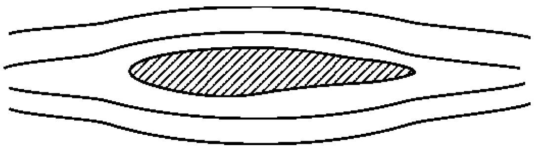
In analysing fluid flow it is useful to visualise the flow pattern. This can be done by drawing lines joining points of equal velocity - velocity contours. These lines are know as streamlines. Here is a simple example of the streamlines around a cross-section of an aircraft wing shaped body:

When fluid is flowing past a solid boundary, e.g. the surface of an aerofoil or the wall of a pipe, fluid obviously does not flow into or out of the surface. So very close to a boundary wall the flow direction must be parallel to the boundary.

i

Close to a solid boundary streamlines are parallel to that boundary
At all points the direction of the streamline is the direction of the fluid velocity: this is how they are defined. Close to the wall the velocity is parallel to the wall so the streamline is also parallel to the wall.

It is also important to recognise that the position of streamlines can change with time - this is the case in unsteady flow. In steady flow, the position of streamlines does not change.

Some things to know about streamlines
ii

Because the fluid is moving in the same direction as the streamlines, fluid can not cross a streamline.
iii

Streamlines can not cross each other. If they were to cross this would indicate two different velocities at the same point. This is not physically possible.
iv

The above point implies that any particles of fluid starting on one streamline will stay on that same streamline throughout the fluid.

A useful technique in fluid flow analysis is to consider only a part of the total fluid in isolation from the rest. This can be done by imagining a tubular surface formed by streamlines along which the fluid flows. This tubular surface is known as a streamtube.

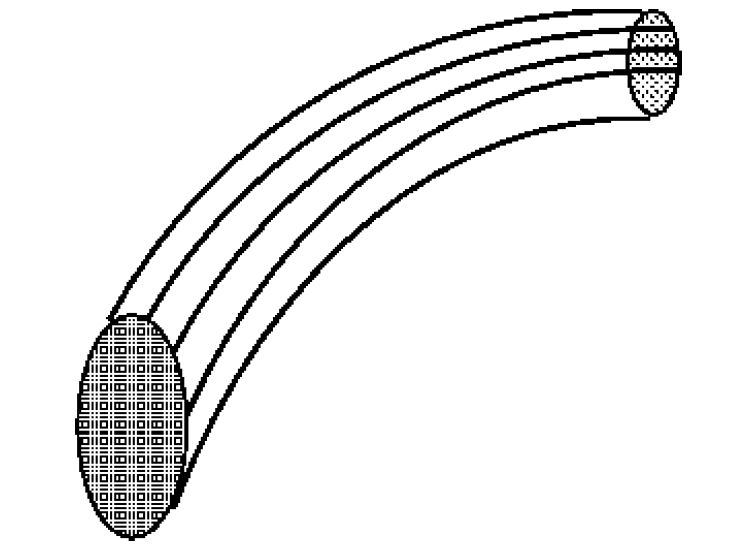
And in a two-dimensional flow we have a streamtube which is flat (in the plane of the paper):

The ”walls” of a streamtube are made of streamlines. As we have seen above, fluid cannot flow across a streamline, so fluid cannot cross a streamtube wall. The streamtube can often be viewed as a solid walled pipe. A streamtube is not a pipe - it differs in unsteady flow as the walls will move with time. And it differs because the ”wall” is moving with the fluid

4.5 Continuity and Conservation of Matter

4.5.1 Flow rate: Mass flow rate

If we want to measure the rate at which water is flowing along a pipe. A very simple way of doing this is to catch all the water coming out of the pipe in a bucket over a fixed time period. Measuring the weight of the water in the bucket and dividing this by the time taken to collect this water gives a rate of accumulation of mass. This is know as the mass flow rate.

For example an empty bucket weighs $2.0kg$ . After 7 seconds of collecting water the bucket weighs $8.0kg$ , then:

	mass flow rate	$\displaystyle=\dot{m}=\frac{\text{mass of fluid in the bucket}}{\text{time % taken to collect the fluid}}$
		$\displaystyle=\frac{8.0-2.0}{7}$
		$\displaystyle=0.857\;kg/s\qquad(kg\;s^{-1})$

Performing a similar calculation, if we know the mass flow is $1.7\;kg/s$ , how long will it take to fill a container with $8\;kg$ of fluid?

	tiem	$\displaystyle=\frac{\text{mass}}{\text{mass flow rate}}$
		$\displaystyle=\frac{8.0}{1.7}$
		$\displaystyle=4.7\;s$

4.5.2 Flow rate: Volume flow rate - Discharge.

More commonly we need to know the volume flow rate - this is more commonly know as discharge. (It is also commonly, but inaccurately, simply called flow rate). The symbol normally used for discharge is $Q$ . The discharge is the volume of fluid flowing per unit time. Multiplying this by the density of the fluid gives us the mass flow rate. Consequently, if the density of the fluid in the above example is $850\;kg\;m^{-3}$ then:

	$\displaystyle\text{discharge }Q$	$\displaystyle=\frac{\text{volume of fluid}}{\text{time}}$
		$\displaystyle=\frac{\text{mass of fluid}}{\text{density }\times\text{ time}}$
		$\displaystyle=\frac{\text{mass flow rate}}{\text{density}}$
		$\displaystyle=\frac{0.857}{850}$
		$\displaystyle=0.001008\;m^{3}/s\qquad(m^{3}\;s^{-1})$
		$\displaystyle=1.0\times 10^{-3}\;m^{3}$
		$\displaystyle=1.008\;litres/s\qquad(l\;s^{-1})$

An important aside about units should be made here:

As has already been stressed, we must always use a consistent set of units when applying values to equations. It would make sense therefore to always quote the values in this consistent set. This set of units will be the SI units. Unfortunately, and this is the case above, these actual practical values are very small or very large ( $0.001008\;m^{3}/s$ is very small). These numbers are difficult to imagine physically. In these cases it is useful to use derived units, and in the case above the useful derived unit is the $litre$ .

( $1\;litre=1.0\times 10^{-3}\;m^{3}$ ). So the solution becomes $1.008\;l/s$ . It is far easier to imagine $1\;litre$ than $1.0\times 10^{-3}\;m^{3}$ . Units must always be checked, and converted if necessary to a consistent set before using in an equation.

4.5.3 Discharge and mean velocity.

If we know the size of a pipe, and we know the discharge, we can deduce the mean velocity

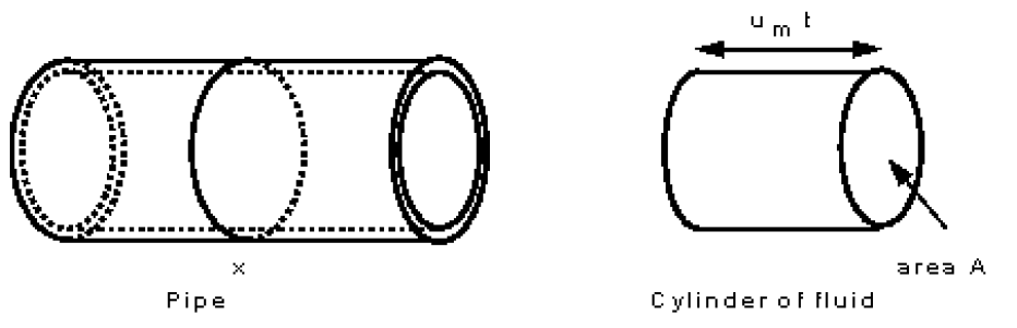
If the area of cross section of the pipe at point $X$ is $A$ , and the mean velocity here is $u_{m}$ . During a time $t$ , a cylinder of fluid will pass point $X$ with a volume $A\times u_{m}\times t$ . The volume per unit time (the discharge) will thus be

	$\displaystyle Q$	$\displaystyle=\frac{\text{volume}}{\text{time}}=\frac{A\times u_{m}\times t}{t}$
	$\displaystyle Q$	$\displaystyle=Au_{m}$

So if the cross-section area, $A$ , is $1.2\times 10^{-3}\;m^{2}$ and the discharge, $Q$ is $24\;l/s$ , then the mean velocity, $u_{m}$ , of the fluid is

	$\displaystyle u_{m}$	$\displaystyle=\frac{Q}{A}$
		$\displaystyle=\frac{2.4\times 10^{-3}}{1.2\times 10^{-3}}$
		$\displaystyle=2.0\;m/s$

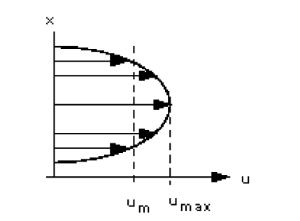
Note how carefully we have called this the mean velocity. This is because the velocity in the pipe is not constant across the cross section. Crossing the centreline of the pipe, the velocity is zero at the walls increasing to a maximum at the centre then decreasing symmetrically to the other wall. This variation across the section is known as the velocity profile or distribution. A typical one is shown in the figure below.

This idea, that mean velocity multiplied by the area gives the discharge, applies to all situations - not just pipe flow.

4.6 Continuity

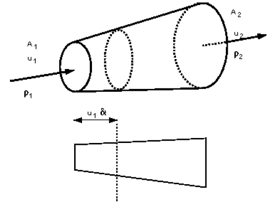
Matter cannot be created or destroyed - (it is simply changed in to a different form of matter). This principle is know as the conservation of mass and we use it in the analysis of flowing fluids.

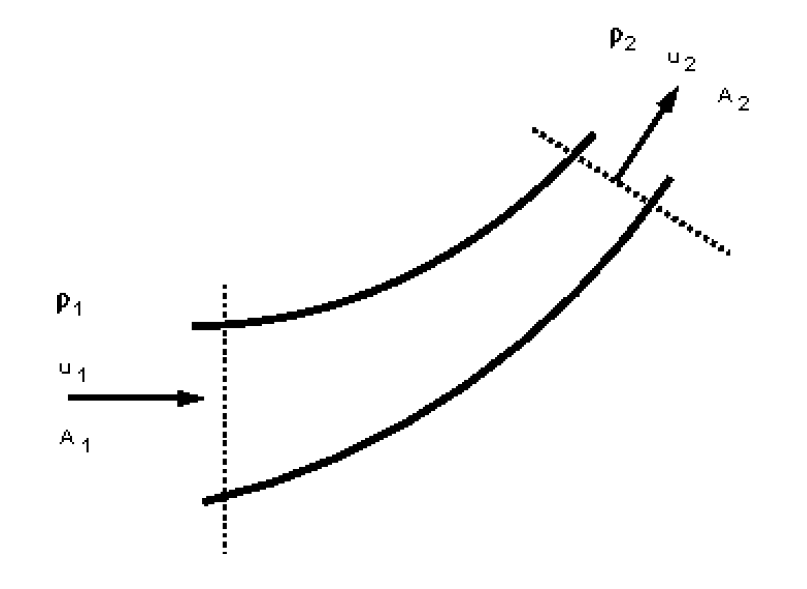
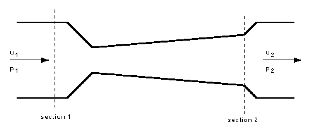
The principle is applied to fixed volumes, known as control volumes (or surfaces), like that in the figure below:

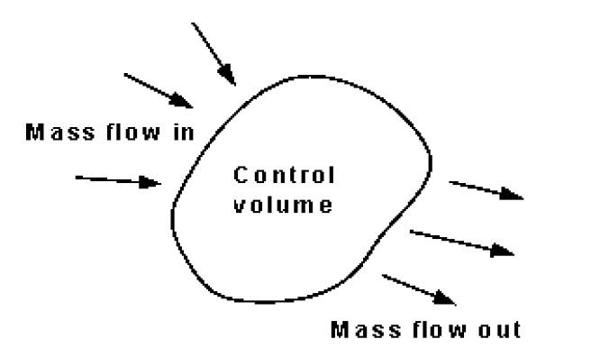
For any control volume the principle of conservation of mass says

Mass entering per unit time = Mass leaving per unit time + Increase of mass in the control volume per unit time

For steady flow there is no increase in the mass within the control volume, so

For steady flow Mass entering per unit time = Mass leaving per unit time

This can be applied to a streamtube such as that shown below. No fluid flows across the boundary made by the streamlines so mass only enters and leaves through the two ends of this streamtube section.

We can then write

	mass entering per unit time at end 1	$\displaystyle=\text{mass leaving per unit time at end 2}$
	$\displaystyle\rho_{1}\delta A_{1}u_{1}$	$\displaystyle=\rho_{2}\delta A_{2}u_{2}$

Or for steady flow,

\rho_{1}\delta A_{1}u_{1}=\rho_{2}\delta A_{2}u_{2}=\text{Constant}=\dot{m}

This is the equation of continuity.

The flow of fluid through a real pipe (or any other vessel) will vary due to the presence of a wall - in this case we can use the mean velocity and write

\rho_{1}A_{1}u_{m1}=\rho_{2}A_{2}u_{m2}=\text{Constant}=\dot{m}

When the fluid can be considered incompressible, i.e. the density does not change, $\rho$ 1 = $\rho$ 2 = $\rho$ so (dropping the m subscript)

A_{1}u_{1}=A_{2}u_{2}=Q

This is the form of the continuity equation most often used.

This equation is a very powerful tool in fluid mechanics and will be used repeatedly throughout the rest of this course.

Some example applications

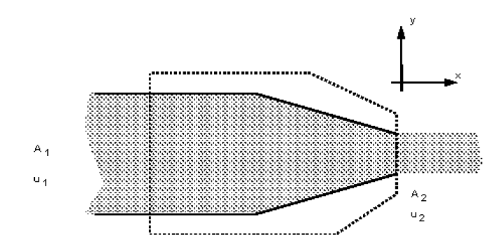
We can apply the principle of continuity to pipes with cross sections which change along their length. Consider the diagram below of a pipe with a contraction:

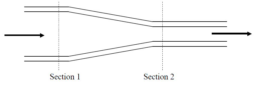
A liquid is flowing from left to right and the pipe is narrowing in the same direction. By the continuity principle, the mass flow rate must be the same at each section - the mass going into the pipe is equal to the mass going out of the pipe. So we can write:

A_{1}u_{1}\rho_{1}=A_{2}u_{2}\rho_{2}

(with the sub-scripts 1 and 2 indicating the values at the two sections)

As we are considering a liquid, usually water, which is not very compressible, the density changes very little so we can say $\rho_{1}=\rho_{2}=\rho$ . This also says that the volume flow rate is constant or that

	Discharge at section 1	$\displaystyle=\text{Discharge at section 2}$
	$\displaystyle Q_{1}$	$\displaystyle=Q_{2}$
	$\displaystyle A_{1}u_{1}$	$\displaystyle=A_{2}u_{2}$

For example if the area $A_{1}=10\times 10^{-3}m^{2}$ and $A_{2}=3\times 10^{-3}m^{2}$ and the upstream mean velocity, $u_{1}=2.1m/s$ , then the downstream mean velocity can be calculated by

	$\displaystyle u_{2}$	$\displaystyle=\frac{A_{1}u_{1}}{A_{2}}$
		$\displaystyle=7.0m/s$

Notice how the downstream velocity only changes from the upstream by the ratio of the two areas of the pipe. As the area of the circular pipe is a function of the diameter we can reduce the calculation further,

	$\displaystyle u_{2}$	$\displaystyle=\frac{A_{1}}{A_{2}}u_{1}=\frac{\pi d^{2}_{1}/4}{\pi d^{2}_{2}/4}% u_{1}=\frac{d^{2}_{1}}{d^{2}_{1}u_{1}}$
		$\displaystyle=(\frac{d_{1}}{d_{2}})^{2}u_{1}$

Now try this on a diffuser, a pipe which expands or diverges as in the figure below,

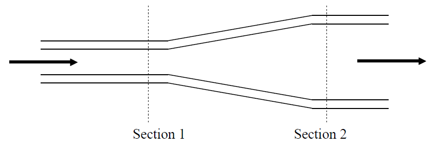
If the diameter at section 1 is $d_{1}=30mm$ and at section 2 $d_{2}=40mm$ and the mean velocity at section 2 is $u_{2}=3.0m/s$ . The velocity entering the diffuser is given by,

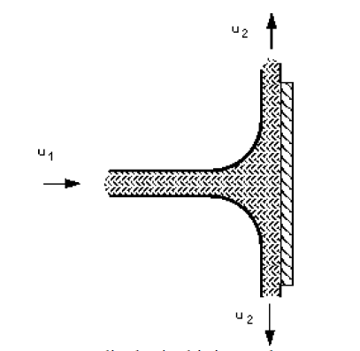
	$\displaystyle u_{1}$	$\displaystyle=(\frac{40}{30})^{2}3.0$
		$\displaystyle=5.3m/s$

Another example of the use of the continuity principle is to determine the velocities in pipes coming from a junction.

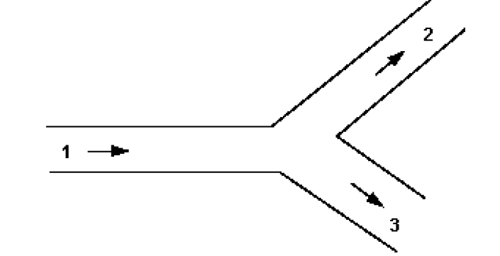
Total mass flow into the junction = Total mass flow out of the junction

\centering\rho_{1}Q_{1}=\rho_{2}Q_{2}+\rho_{3}Q_{3}\@add@centering

When the flow is incompressible (e.g. if it is water) $\rho_{1}$ = $\rho_{2}$ = $\rho$

\displaystyle Q_{1}

\displaystyle=Q_{2}+Q_{3}A_{1}u_{1}

\displaystyle=A_{2}u_{2}+A_{3}u_{3}

If pipe 1 diameter = 50mm, mean velocity 2m/s, pipe 2 diameter 40mm takes 30% of total discharge and pipe 3 diameter 60mm. What are the values of discharge and mean velocity in each pipe?

	$\displaystyle Q_{1}$	$\displaystyle=A_{1}u_{1}=(\frac{\pi d^{2}}{4})u$
		$\displaystyle=0.00392m^{3}/s$

	$\displaystyle Q_{2}$	$\displaystyle=0.3Q_{1}=0.001178m^{3}/s$
	$\displaystyle Q_{1}$	$\displaystyle=Q_{2}+Q_{3}$
	$\displaystyle Q_{3}$	$\displaystyle=Q_{1}-0.3Q_{1}=0.7Q_{1}$
		$\displaystyle=0.00275m^{3}/s$

	$\displaystyle Q_{2}$	$\displaystyle=A_{2}u_{2}$
	$\displaystyle u_{2}$	$\displaystyle=0.936m/s$

	$\displaystyle Q_{3}$	$\displaystyle=A_{3}u_{3}$
	$\displaystyle u_{3}$	$\displaystyle=0.972m/s$

4.7 The Bernoulli equation

4.7.1 Work and energy

We know that if we drop a ball it accelerates downward with an acceleration $g=9.81m/s^{2}$ (neglecting the frictional resistance due to air). We can calculate the speed of the ball after falling a distance h by the formula $v^{2}=u^{2}+2as$ (a = g and s = h). The equation could be applied to a falling droplet of water as the same laws of motion apply

A more general approach to obtaining the parameters of motion (of both solids and fluids) is to apply the principle of conservation of energy. When friction is negligible the

sum of kinetic energy and gravitational potential energy is constant.

Kinetic energy $=\frac{1}{2}mv^{2}$

Gravitational potential energy $=mgh$

(m is the mass, v is the velocity and h is the height above the datum).

To apply this to a falling droplet we have an initial velocity of zero, and it falls through a height of h.

Initial kinetic energy $=0$

Initial potential energy $=mgh$

Final kinetic energy $=\frac{1}{2}mv^{2}$

Final potential energy $=0$

We know that

kinetic energy + potential energy = constant

so

Initial kinetic energy + Initial potential energy = Final kinetic energy + Final potential energy

mgh=\frac{1}{2}mv^{2}

so

v=\sqrt{2gh}

Although this is applied to a drop of liquid, a similar method can be applied to a continuous jet of liquid.

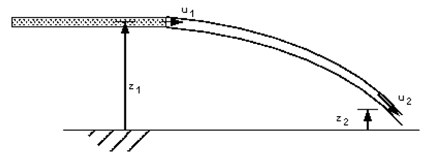
We can consider the situation as in the figure above - a continuous jet of water coming from a pipe with velocity $u_{1}$ . One particle of the liquid with mass $m$ travels with the jet and falls from height $z_{1}$ to $z_{2}$ . The velocity also changes from $u_{1}$ to $u_{2}$ . The jet is travelling in air where the pressure is everywhere atmospheric so there is no force due to pressure acting on the fluid. The only force which is acting is that due to gravity. The sum of the kinetic and potential energies remains constant (as we neglect energy losses due to friction) so

mgz_{1}+\frac{1}{2}mu^{2}_{1}=mgz_{2}+\frac{1}{2}mu^{2}_{2}

As is constant this becomes

\frac{1}{2}u^{2}_{1}+gz_{1}=\frac{1}{2}u^{2}_{2}+gz_{2}

This will give a reasonably accurate result as long as the weight of the jet is large compared to the frictional forces. It is only applicable while the jet is whole - before it breaks up into droplets.

Flow from a reservoir

We can use a very similar application of the energy conservation concept to determine the velocity of flow along a pipe from a reservoir. Consider the ’idealised reservoir’ in the figure below.

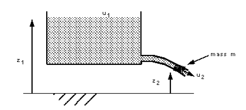
The level of the water in the reservoir is $z_{1}$ . Considering the energy situation - there is no movement of water so kinetic energy is zero but the gravitational potential energy is $mgz_{1}$ . If a pipe is attached at the bottom water flows along this pipe out of the tank to a level $z_{2}$ . A mass $m$ has flowed from the top of the reservoir to the nozzle and it has gained a velocity $u_{2}$ . The kinetic energy is now $\frac{1}{2}mu^{2}_{2}$ and the potential energy $mgz_{2}$ . Summarising

Initial kinetic energy $=0$
Initial potential energy $=mgz_{1}$
Final kinetic energy $=\frac{1}{2}mu^{2}_{2}$
Final potential energy $=mgz_{2}$

We know that

kinetic energy + potential energy = constant

so

	$\displaystyle mgz_{1}$	$\displaystyle=\frac{1}{2}mu^{2}_{2}+mgz_{2}$
	$\displaystyle mg(z_{1}+z_{2})$	$\displaystyle=\frac{1}{2}mu^{2}_{2}$

so

u_{2}=\sqrt{2g(z_{1}-z_{2})}

We now have a expression for the velocity of the water as it flows from of a pipe nozzle at a height $(z_{1}-z_{2})$ below the surface of the reservoir. (Neglecting friction losses in the pipe and the nozzle).

Now apply this to this example: A reservoir of water has the surface at 310m above the outlet nozzle of a pipe with diameter 15mm. What is the a) velocity, b) the discharge out of the nozzle and c) mass flow rate. (Neglect all friction in the nozzle and the pipe).

	$\displaystyle u_{2}$	$\displaystyle=\sqrt{2g(z_{1}-z_{2})}$
		$\displaystyle=\sqrt{2\times g\times 310}$
		$\displaystyle=78.0$

Volume flow rate is equal to the area of the nozzle multiplied by the velocity

	$\displaystyle Q$	$\displaystyle=Au$
		$\displaystyle=(\pi\times\frac{0.015^{2}}{4})\times 78.0$
		$\displaystyle=0.01378m^{3}/s$

The density of water is $1000kg/m^{3}$ so the mass flow rate is

	mass flow rate	$\displaystyle=\text{density}\times\text{volume flow rate}$
		$\displaystyle=\rho Q$
		$\displaystyle=1000\times 0.01378$
		$\displaystyle=13.78kg/s$

In the above examples the resultant pressure force was always zero as the pressure surrounding the fluid was the everywhere the same - atmospheric. If the pressures had been different there would have been an extra force acting and we would have to take into account the work done by this force when calculating the final velocity.

We have already seen in the hydrostatics section an example of pressure difference where the velocities are zero.

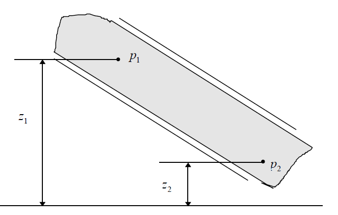
The pipe is filled with stationary fluid of density $\rho$ has pressures $\rho_{1}$ and $zrho_{2}$ at levels $z_{1}$ and $z_{2}$ respectively. What is the pressure difference in terms of these levels?

p_{2}-p_{1}=\rho g(z_{1}-z_{2})

or

\frac{p_{1}}{\rho}+gz_{1}=\frac{P_{2}}{\rho}+gz_{2}

This applies when the pressure varies but the fluid is stationary.

Compare this to the equation derived for a moving fluid but constant pressure:

\frac{1}{2}u^{2}_{1}+gz_{1}=\frac{1}{2}u^{2}_{2}+gz_{2}

You can see that these are similar form. What would happen if both pressure and velocity varies?

4.8 Bernoulli’s Equation

Bernoulli’s equation is one of the most important/useful equations in fluid mechanics. It may be written,

\frac{p_{1}}{\rho g}+\frac{u^{2}_{1}}{2g}+z_{1}=\frac{p_{2}}{\rho g}+\frac{u^{% 2}_{2}}{2g}+z_{2}

The Bernoulli Equation

We see that from applying equal pressure or zero velocities we get the two equations from the section above. They are both just special cases of Bernoulli’s equation.

Bernoulli’s equation has some restrictions in its applicability, they are: The Bernoulli equation applies when:

1.

Flow is steady;
2.

Density is constant (which also means the fluid is incompressible);
3.

Friction losses are negligible.
4.

The equation relates the states at two points along a single streamline, (not conditions on two different streamlines).

All these conditions are impossible to satisfy at any instant in time! Fortunately for many real situations where the conditions are approximately satisfied, the equation gives very good results.

The derivation of Bernoulli’s Equation:

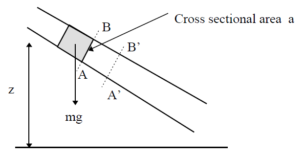
An element of fluid, as that in the figure above, has potential energy due to its height $z$ above a datum and kinetic energy due to its velocity $u$ . If the element has weight $mg$ then

potential energy $=mgz$
potential energy per unit weight $=z$

and

kinetic energy $=\frac{1}{2}mu^{2}$
kinetic energy per unit weight $=\frac{u^{2}}{2g}$

At any cross-section the pressure generates a force, the fluid will flow, moving the cross-section, so work will be done. If the pressure at cross section AB is $p$ and the area of the cross-section is $a$ then

\text{force on AB}=pa

when the mass $mg$ of fluid has passed AB, cross-section AB will have moved to A’B’

\text{volume passing AB }=\frac{mg}{\rho g}=\frac{m}{\rho}

therefore

\text{distance AA'}=\frac{m}{\rho a}

and

	work done	$\displaystyle=\text{force }\times\text{distance AA'}$
		$\displaystyle=pa\times\frac{m}{\rho a}=\frac{pm}{\rho}$

\text{work done per unit weight}=\frac{p}{\rho g}

This term is know as the pressure energy of the flowing stream.

Summing all of these three energy terms gives

Pressure		Kinetic		Potential		Total
energy per	+	energy per	+	energy per	=	energy per
unit weight		unit weight		unit weight		unit weight

or

\frac{p}{\rho g}+\frac{u^{2}}{2g}+z=H

As all of these elements of the equation have units of length, they are often referred to as the following:

	pressure head	$\displaystyle=\frac{p}{\rho g}$
	velocity head	$\displaystyle=\frac{u^{2}}{2g}$
	potential head	$\displaystyle=z$
	total head	$\displaystyle=H$

By the principle of conservation of energy the total energy in the system does not change. Thus the total head does not change. So the Bernoulli equation can be written

\frac{p}{\rho g}+\frac{u^{2}}{2g}+z=H=\text{constant}

As stated above, the Bernoulli equation applies to conditions along a streamline. We can apply it between two points, 1 and 2, on the streamline in the figure below

\text{total energy per unit weight at 1 }=\text{total energy per unit weight % at 2}

or

\text{total head at 1}=\text{total head at 2}

or

\frac{p_{1}}{\rho g}+\frac{u^{2}_{1}}{2g}+z_{1}=\frac{p_{2}}{\rho g}+\frac{u^{% 2}_{2}}{2g}+z_{2}

This equation assumes no energy losses (e.g. from friction) or energy gains (e.g. from a pump) along the streamline. It can be expanded to include these simply, by adding the appropriate energy terms:

Total		Total		Loss of		Work done		Eneergy
energy per	=	energy per	+	energy per	+	per	-	supplied
unit weight at 1		unit weight at 2		unit weight, $h$		unit weight, $w$		per unit weight, $q$

or

\left(\frac{p_{1}}{\rho g}+\frac{u^{2}_{1}}{2g}+z_{1}\right)=\left(\frac{p_{2}% }{\rho g}+\frac{u^{2}_{2}}{2g}+z_{2}\right)+h+w-q

4.8.1 An example of the use of the Bernoulli equation.

When the Bernoulli equation is combined with the continuity equation the two can be used to find velocities and pressures at points in the flow connected by a streamline.

Here is an example of using the Bernoulli equation to determine pressure and velocity at within a contracting and expanding pipe.

A fluid of constant density $\rho=960kg/m^{3}$ is flowing steadily through the above tube. The diameters at the sections are $d_{1}=100mm$ and $d_{2}=80mm$ . The gauge pressure at 1 is $p_{1}=200kN/m^{2}$ and the velocity here is $u_{1}=5m/s$ . We want to know the gauge pressure at section 2.

We shall of course use the Bernoulli equation to do this and we apply it along a streamline joining section 1 with section 2.

The tube is horizontal, with $z_{1}=z_{2}$ so Bernoulli gives us the following equation for pressure at section 2:

p_{2}=p_{1}+\frac{\rho}{2}\left(u^{2}_{1}-u^{2}_{2}\right)

But we do not know the value of $u_{2}$ . We can calculate this from the continuity equation: Discharge into the tube is equal to the discharge out i.e.

	$\displaystyle A_{1}u_{1}$	$\displaystyle=A_{2}u_{2}$
	$\displaystyle u_{2}$	$\displaystyle=\frac{A_{1}u_{1}}{A_{2}}$
	$\displaystyle u_{2}$	$\displaystyle=\left(\frac{d_{1}}{d_{2}}\right)^{2}u_{1}$
		$\displaystyle=7.8125m/s$

So we can now calculate the pressure at section 2

	$\displaystyle p_{2}$	$\displaystyle=200000-17296.87$
		$\displaystyle=182703N/m^{2}$
		$\displaystyle=182.7kN/m^{2}$

Notice how the velocity has increased while the pressure has decreased. The phenomenon - that pressure decreases as velocity increases - sometimes comes in very useful in engineering. (It is on this principle that carburettor in many car engines work - pressure reduces in a contraction allowing a small amount of fuel to enter).

Here we have used both the Bernoulli equation and the Continuity principle together to solve the problem. Use of this combination is very common. We will be seeing this again frequently throughout the rest of the course.

4.9 Pressure Head, Velocity Head, Potential Head and Total Head.

By looking again at the example of the reservoir with which feeds a pipe we will see how these different heads relate to each other.

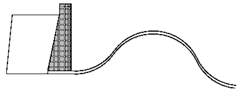
Consider the reservoir below feeding a pipe which changes diameter and rises (in reality it may have to pass over a hill) before falling to its final level.

To analyses the flow in the pipe we apply the Bernoulli equation along a streamline from point 1 on the surface of the reservoir to point 2 at the outlet nozzle of the pipe. And we know that the total energy per unit weight or the total head does not change - it is constant - along a streamline. But what is this value of this constant? We have the Bernoulli equation

\frac{p_{1}}{\rho g}+\frac{u^{2}_{1}}{2g}+z_{1}=H=\frac{p_{2}}{\rho g}+\frac{u% ^{2}_{2}}{2g}+z_{2}

We can calculate the total head, H, at the reservoir, $p_{1}=0$ as this is atmospheric and atmospheric gauge pressure is zero, the surface is moving very slowly compared to that in the pipe so $u_{1}=0$ , so all we are left with is total head = $H=z_{1}$ the elevation of the reservoir. A useful method of analysing the flow is to show the pressures graphically on the same diagram as the pipe and reservoir. In the figure above the total head line is shown. If we attached piezometers at points along the pipe, what would be their levels when the pipe nozzle was closed? (Piezometers, as you will remember, are simply open ended vertical tubes filled with the same liquid whose pressure they are measuring).

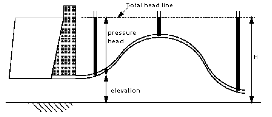
As you can see in the above figure, with zero velocity all of the levels in the piezometers are equal and the same as the total head line. At each point on the line, when $u=0$

\frac{p}{\rho g}+z=H

The level in the piezometer is the pressure head and its value is given by $\frac{p}{\rho g}$ . What would happen to the levels in the piezometers (pressure heads) if the if water was flowing with velocity $=u$ ? We know from earlier examples that as velocity increases so pressure falls…

\frac{p}{\rho g}+\frac{u^{2}}{2g}+\ =H

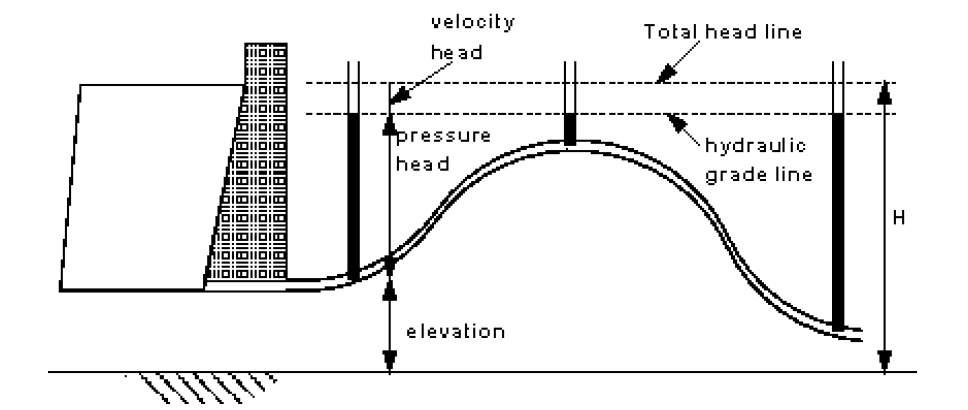
We see in this figure that the levels have reduced by an amount equal to the velocity head, $\frac{u^{2}}{2g}$ . Now as the pipe is of constant diameter we know that the velocity is constant along the pipe so the velocity head is constant and represented graphically by the horizontal line shown. (this line is known as the hydraulic grade line).

What would happen if the pipe were not of constant diameter? Look at the figure below where the pipe from the example above is replaced be a pipe of three sections with the middle section of larger diameter

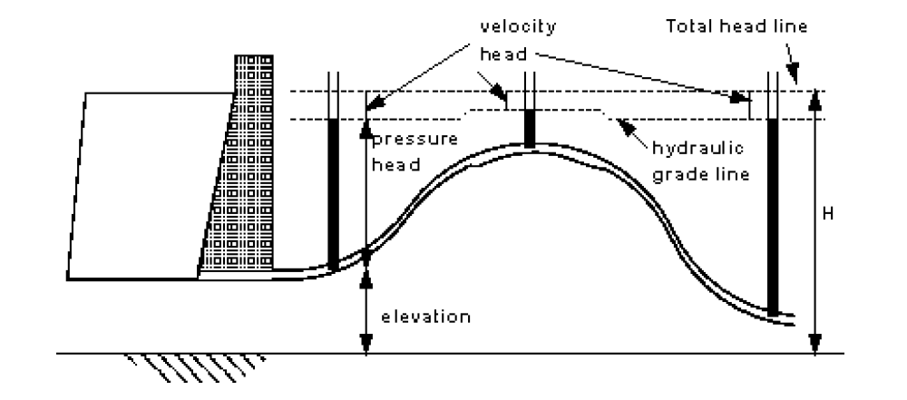
The velocity head at each point is now different. This is because the velocity is different at each point. By considering continuity we know that the velocity is different because the diameter of the pipe is different. Which pipe has the greatest diameter?

Pipe 2, because the velocity, and hence the velocity head, is the smallest.

This graphical representation has the advantage that we can see at a glance the pressures in the system. For example, where along the whole line is the lowest pressure head? It is where the hydraulic grade line is nearest to the pipe elevation i.e. at the highest point of the pipe.

4.10 Losses due to friction.

In a real pipe line there are energy losses due to friction - these must be taken into account as they can be very significant. How would the pressure and hydraulic grade lines change with friction? Going back to the constant diameter pipe, we would have a pressure situation like this shown below

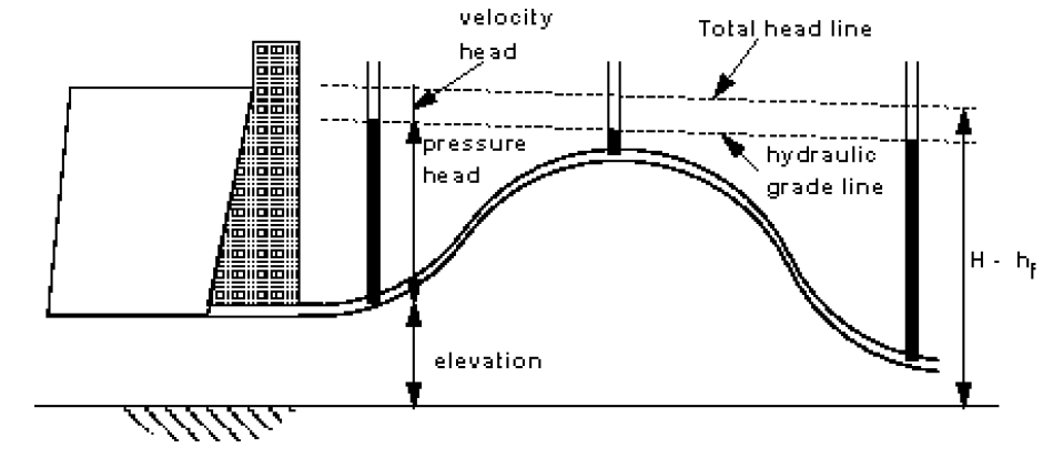
How can the total head be changing? We have said that the total head - or total energy per unit weight - is constant. We are considering energy conservation, so if we allow for an amount of energy to be lost due to friction the total head will change. We have seen the equation for this before. But here it is again with the energy loss due to friction written as a head and given the symbol $h_{f}$ . This is often know as the head loss due to friction.

\frac{p_{1}}{\rho g}+\frac{u^{2}_{1}}{2g}+z_{1}=\frac{p_{2}}{\rho g}+\frac{u^{% 2}_{2}}{2g}+z_{2}+h_{f}

4.11 Applications of the Bernoulli Equation

The Bernoulli equation can be applied to a great many situations not just the pipe flow we have been considering up to now. In the following sections we will see some examples of its application to flow measurement from tanks, within pipes as well as in open channels.

4.11.1 Pitot Tube

If a stream of uniform velocity flows into a blunt body, the stream lines take a pattern similar to this:

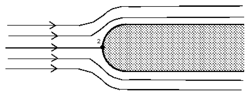
Note how some move to the left and some to the right. But one, in the centre, goes to the tip of the blunt body and stops. It stops because at this point the velocity is zero - the fluid does not move at this one point. This point is known as the stagnation point.

From the Bernoulli equation we can calculate the pressure at this point. Apply Bernoulli along the central streamline from a point upstream where the velocity is $u_{1}$ and the pressure $p_{1}$ to the stagnation point of the blunt body where the velocity is zero, $u_{2}=0$ . Also $z1=z2$ .

	$\displaystyle\frac{p_{1}}{\rho g}+\frac{u^{2}_{1}}{2g}+z_{1}$	$\displaystyle=\frac{p_{2}}{\rho g}+\frac{u^{2}_{2}}{2g}+z_{2}$
	$\displaystyle\frac{p_{1}}{\rho}+\frac{u^{2}_{1}}{2}$	$\displaystyle=\frac{p_{2}}{\rho}$
	$\displaystyle p_{2}$	$\displaystyle=p_{1}+\frac{1}{2}\rho u^{2}_{1}$

This increase in pressure which bring the fluid to rest is called the dynamic pressure.

Dynamic pressure = $\frac{1}{2}\rho u^{2}_{1}$

or converting this to head (using $h=\frac{p}{\rho g}$ )

Dynamic head = $\frac{1}{2g}u^{2}_{1}$

The total pressure is know as the stagnation pressure (or total pressure)

Stagnation pressure = $p_{1}+\frac{1}{2}\rho u^{2}_{1}$

or in terms of head

Stagnation head = $\frac{p_{1}}{\rho g}+\frac{1}{2g}u^{2}_{1}$

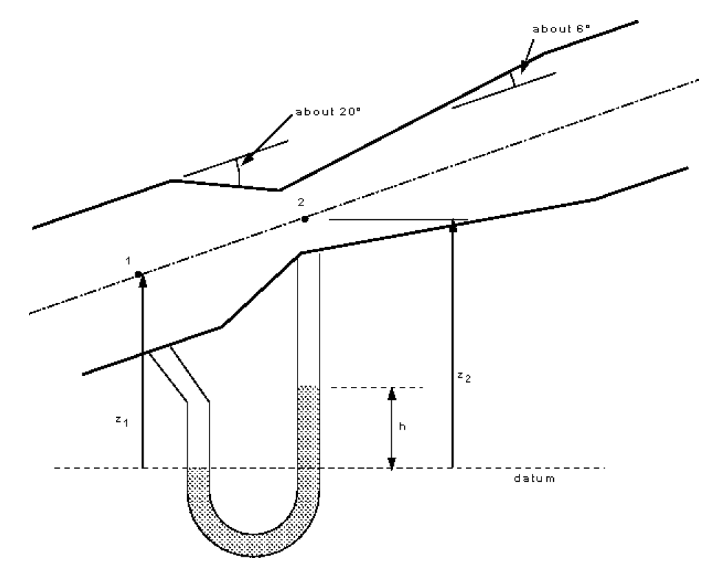
The blunt body stopping the fluid does not have to be a solid. I could be a static column of fluid. Two piezometers, one as normal and one as a Pitot tube within the pipe can be used in an arrangement shown below to measure velocity of flow.

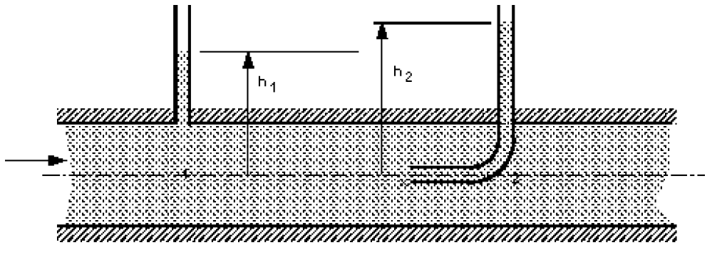
Using the above theory, we have the equation for $p_{2}$ ,

	$\displaystyle p_{2}$	$\displaystyle=p_{1}+\frac{1}{2}\rho u^{2}_{1}$
	$\displaystyle\rho gh_{2}$	$\displaystyle=\rho gh_{1}+\frac{1}{2}\rho u^{2}_{1}$
	$\displaystyle u$	$\displaystyle=\sqrt{2g(h_{2}-h_{1})}$

We now have an expression for velocity obtained from two pressure measurements and the application of the Bernoulli equation.

4.12 Pitot Static Tube

The necessity of two piezometers and thus two readings make this arrangement a little awkward. Connecting the piezometers to a manometer would simplify things but there are still two tubes. The Pitot static tube combines the tubes and they can then be easily connected to a manometer. A Pitot static tube is shown below. The holes on the side of the tube connect to one side of a manometer and register the static head, ( $h_{1}$ ), while the central hole is connected to the other side of the manometer to register, as before, the stagnation head ( $h_{2}$ ).

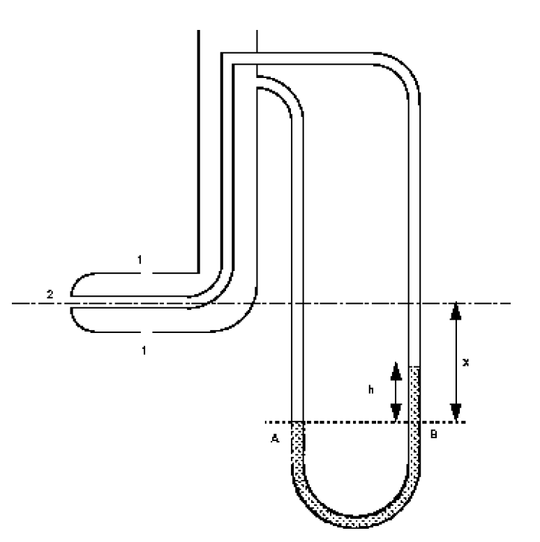
Consider the pressures on the level of the centre line of the Pitot tube and using the theory of the manometer,

	$\displaystyle p_{A}$	$\displaystyle=p_{2}+\rho gX$
	$\displaystyle p_{B}$	$\displaystyle=p_{1}+\rho g(X-h)+\rho_{man}gh$
	$\displaystyle p_{A}$	$\displaystyle=p_{B}$
	$\displaystyle p_{2}+\rho gX$	$\displaystyle=p_{1}+\rho g(X-h)+\rho_{man}gh$

We know that $p_{2}=p_{static}=p_{1}+\frac{1}{2}\rho u^{2}_{1}$ , substituting this in to the above gives

	$\displaystyle p_{1}+hg(\rho_{man}-\rho)$	$\displaystyle=p_{1}+\frac{\rho u^{2}_{1}}{2}$
	$\displaystyle u_{1}$	$\displaystyle=\sqrt{\frac{2gh(\rho_{m}-\rho)}{\rho}}$

The Pitot/Pitot-static tubes give velocities at points in the flow. It does not give the overall discharge of the stream, which is often what is wanted. It also has the drawback that it is liable to block easily, particularly if there is significant debris in the flow.

4.13 Venturi Meter

The Venturi meter is a device for measuring discharge in a pipe. It consists of a rapidly converging section which increases the velocity of flow and hence reduces the pressure. It then returns to the original dimensions of the pipe by a gently diverging ’diffuser’ section. By measuring the pressure differences the discharge can be calculated. This is a particularly accurate method of flow measurement as energy loss are very small.

Applying Bernoulli along the streamline from point 1 to point 2 in the narrow throat of the Venturi meter we have

\frac{p_{1}}{\rho g}+\frac{u^{2}_{1}}{2g}+z_{1}=\frac{p_{2}}{\rho g}+\frac{u^{% 2}_{2}}{2g}+z_{2}

By the using the continuity equation we can eliminate the velocity $u_{2}$ ,

	$\displaystyle Q$	$\displaystyle=u_{1}A_{1}=u_{2}A_{2}$
	$\displaystyle u_{2}$	$\displaystyle=\frac{u_{1}A_{1}}{A_{2}}$

Substituting this into and rearranging the Bernoulli equation we get

\frac{p_{1}-p_{2}}{\rho g}+z_{1}-z_{2}=\frac{u^{2}_{1}}{2g}\left[\left(\frac{A% _{1}}{A_{2}}\right)^{2}-1\right]

u_{1}=\sqrt{\frac{2g\left[\frac{p_{1}-p_{2}}{\rho g}+z_{1}-z_{2}\right]}{\left% (\frac{A_{1}}{A_{2}}\right)^{2}-1}}

To get the theoretical discharge this is multiplied by the area. To get the actual discharge taking in to account the losses due to friction, we include a coefficient of discharge

	$\displaystyle Q_{\text{ideal}}$	$\displaystyle=u_{1}A_{1}$
	$\displaystyle Q_{\text{actual}}$	$\displaystyle=C_{d}Q_{\text{ideal}}=C_{d}u_{1}A_{1}$
	$\displaystyle Q_{\text{actual}}$	$\displaystyle=C_{d}A_{1}A_{2}\sqrt{\frac{2g\left[\frac{p_{1}-p_{2}}{\rho g}+z_% {1}-z_{2}\right]}{A^{2}_{1}-A^{2}_{2}}}$

This can also be expressed in terms of the manometer readings

	$\displaystyle p_{1}+\rho gz_{1}$	$\displaystyle=p_{2}+\rho_{man}gh+\rho g(z_{2}-h)$
	$\displaystyle\frac{p_{1}-p_{2}}{\rho g}+z_{1}-z_{2}$	$\displaystyle=h\left(\frac{\rho_{man}}{\rho}-1\right)$

Thus the discharge can be expressed in terms of the manometer reading:

Q_{actual}=C_{d}A_{1}A_{2}\sqrt{\frac{2gh\left(\frac{\rho_{man}}{\rho}-1\right% )}{A^{2}_{1}-A^{2}_{1}}}

Notice how this expression does not include any terms for the elevation or orientation ( $z_{1}$ or $z_{2}$ ) of the Venturimeter. This means that the meter can be at any convenient angle to function.

The purpose of the diffuser in a Venturi meter is to assure gradual and steady deceleration after the throat. This is designed to ensure that the pressure rises again to something near to the original value before the Venturi meter. The angle of the diffuser is usually between 6 and 8 degrees. Wider than this and the flow might separate from the walls resulting in increased friction and energy and pressure loss. If the angle is less than this the meter becomes very long and pressure losses again become significant. The efficiency of the diffuser of increasing pressure back to the original is rarely greater than 80%.

4.14 Flow Through A Small Orifice

We are to consider the flow from a tank through a hole in the side close to the base. The general arrangement and a close up of the hole and streamlines are shown in the figure below

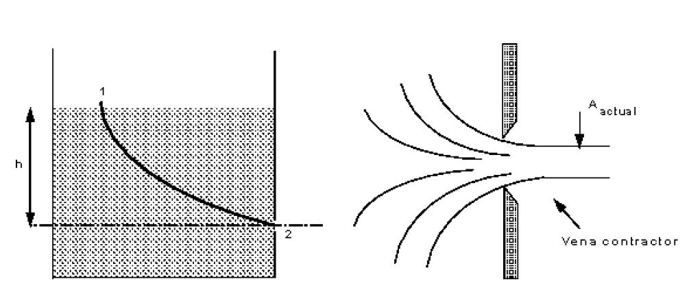
The shape of the holes edges are as they are (sharp) to minimise frictional losses by minimising the contact between the hole and the liquid - the only contact is the very edge.

Looking at the streamlines you can see how they contract after the orifice to a minimum value when they all become parallel, at this point, the velocity and pressure are uniform across the jet. This convergence is called the vena contracta. (From the Latin ’contracted vein’). It is necessary to know the amount of contraction to allow us to calculate the flow.

We can predict the velocity at the orifice using the Bernoulli equation. Apply it along the streamline joining point 1 on the surface to point 2 at the centre of the orifice.

At the surface velocity is negligible ( $u_{1}$ = 0) and the pressure atmospheric ( $p_{1}$ = 0).At the orifice the jet is open to the air so again the pressure is atmospheric ( $p_{2}$ = 0). If we take the datum line through the orifice then $z_{1}=h$ and $z_{2}=0$ , leaving

h=\frac{u^{2}_{2}}{2g}

u_{2}=\sqrt{2gh}

This is the theoretical value of velocity. Unfortunately it will be an over estimate of the real velocity because friction losses have not been taken into account. To incorporate friction we use the coefficient of velocity to correct the theoretical velocity,

u_{\text{actual}}=C_{v}u_{\text{theoretical}}

Each orifice has its own coefficient of velocity, they usually lie in the range( 0.97 - 0.99)

To calculate the discharge through the orifice we multiply the area of the jet by the velocity. The actual area of the jet is the area of the vena contracta not the area of the orifice. We obtain this area by using a coefficient of contraction for the orifice

A_{\text{actual}}=C_{c}A_{\text{orifice}}

So the discharge through the orifice is given by

	$\displaystyle Q$	$\displaystyle=Au$
	$\displaystyle Q_{\text{actual}}$	$\displaystyle=A_{\text{actual}}u_{\text{actual}}$
		$\displaystyle=C_{c}C_{v}A_{\text{orifice}}u_{\text{theoretical}}$
		$\displaystyle=C_{d}A_{\text{orifice}}u_{\text{thoeretical}}$
		$\displaystyle=C_{d}A_{\text{orifice}}\sqrt{2gh}$

Where $C_{d}$ is the coefficient of discharge, and $C_{d}=C_{c}\times C_{v}$

4.15 Time for a Tank to Empty

We now have an expression for the discharge out of a tank based on the height of water above the orifice. It would be useful to know how long it would take for the tank to empty.

As the tank empties, so the level of water will fall. We can get an expression for the time it takes to fall by integrating the expression for flow between the initial and final levels.

The tank has a cross sectional area of $A$ . In a time dt the level falls by $dh$ or the flow out of the tank is

	$\displaystyle Q$	$\displaystyle=Av$
	$\displaystyle Q$	$\displaystyle=-A\frac{\delta h}{\delta t}$

(-ve sign as $\delta h$ is falling)

Rearranging and substituting the expression for Q through the orifice gives

\delta t=\frac{-A}{C_{d}A_{o}\sqrt{2g}}\frac{\delta h}{\sqrt{h}}

This can be integrated between the initial level, $h_{1}$ , and final level, $h_{2}$ , to give an expression for the time it takes to fall this distance

	$\displaystyle t$	$\displaystyle=\frac{-A}{C_{d}A_{o}\sqrt{2g}}\int_{h_{1}}^{h_{2}}\frac{\delta h% }{\sqrt{h}}$
		$\displaystyle=\frac{-A}{C_{d}A_{o}\sqrt{2g}}\left[2\sqrt{h}\right]_{h_{1}}^{h_% {2}}$
		$\displaystyle=\frac{-2A}{C_{d}A_{o}\sqrt{2g}}\left[\sqrt{h_{2}}-\sqrt{h_{1}}\right]$

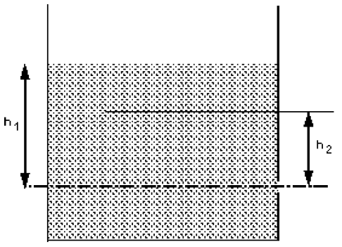
4.15.1 Submerged Orifice

We have two tanks next to each other (or one tank separated by a dividing wall) and fluid is to flow between them through a submerged orifice. Although difficult to see, careful measurement of the flow indicates that the submerged jet flow behaves in a similar way to the jet in air in that it forms a vena contracta below the surface. To determine the velocity at the jet we first use the Bernoulli equation to give us the ideal velocity. Applying Bernoulli from point 1 on the surface of the deeper tank to point 2 at the centre of the orifice, gives

	$\displaystyle\frac{p_{1}}{\rho g}+\frac{u^{2}_{1}}{2g}+z_{1}$	$\displaystyle=\frac{p_{2}}{\rho g}+\frac{u^{2}_{2}}{2g}+z_{2}$
	$\displaystyle 0+0+h_{1}$	$\displaystyle=\frac{\rho gh_{2}}{\rho g}+\frac{u^{2}_{2}}{2g}+0$
	$\displaystyle u_{2}$	$\displaystyle=\sqrt{2g(h_{1}-h_{2})}$

i.e. the ideal velocity of the jet through the submerged orifice depends on the diffenowrence in head across the orifice. And the discharge is given by

	$\displaystyle Q$	$\displaystyle=C_{d}A_{o}u$
		$\displaystyle=C_{d}A_{o}\sqrt{2g(h_{1}-h_{2})}$

4.16 Time for Equalisation of Levels in Two Tanks

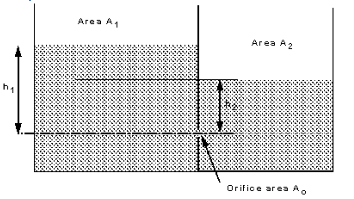
By a similar analysis used to find the time for a level drop in a tank we can derive an expression for the change in levels when there is flow between two connected tanks.

Applying the continuity equation

	$\displaystyle Q$	$\displaystyle=-A_{1}\frac{\delta h_{1}}{\delta t}=\frac{\delta h_{2}}{\delta t}$
	$\displaystyle Q\;\delta t$	$\displaystyle=-A_{1}\delta h_{1}=A_{2}\delta h_{2}$

Also we can write

-\delta h_{1}+\delta h_{2}=\delta h

So

	$\displaystyle-A_{1}\delta h_{1}$	$\displaystyle=A_{2}\left(\delta h_{1}+\delta h\right)$
	$\displaystyle\delta h_{1}$	$\displaystyle=\frac{-A_{2}\delta h}{A_{1}+A_{2}}$

Then we get

	$\displaystyle Q\delta t$	$\displaystyle=-A_{1}\delta h_{1}$
	$\displaystyle C_{d}A_{o}\sqrt{2g(h_{1}-h_{2})}\;\delta t$	$\displaystyle=\frac{A_{1}A_{2}}{A_{1}+A_{2}}\delta h$

Re arranging and integrating between the two levels we get

\delta t=\frac{A_{1}A_{2}}{(A_{1}+A_{2})C_{d}A_{o}\sqrt{2g}}\frac{\delta h}{% \sqrt{h}}

Integrating

	$\displaystyle t$	$\displaystyle=\frac{A_{1}A_{2}}{(A_{1}+A_{2})C_{d}A_{o}\sqrt{2g}}\int_{h_{% \text{initial}}}^{h_{\text{final}}}\frac{1}{\sqrt{h}}\delta h$
		$\displaystyle=\frac{2A_{1}A_{2}}{(A_{1}+A_{2})C_{d}A_{o}\sqrt{2g}}\left[\sqrt{% h}\right]_{h_{\text{initial}}}^{h_{\text{final}}}$
		$\displaystyle=\frac{2A_{1}A_{2}}{(A_{1}+A_{2})C_{d}A_{o}\sqrt{2g}}\left[\sqrt{% h_{\text{initial}}}-\sqrt{h_{\text{final}}}\right]$

(remember that $h$ in this expression is the difference in height between the two levels i.e. $(h_{2}-h_{1})$ to get the time for the levels to equal use $h_{\text{initial}}=h_{1}$ and $h_{\text{final}}=0$ ).

Thus we have an expression giving the time it will take for the two levels to equal.

4.17 Flow Over Notches and Weirs

A notch is an opening in the side of a tank or reservoir which extends above the surface of the liquid. It is usually a device for measuring discharge. A weir is a notch on a larger scale - usually found in rivers. It may be sharp crested but also may have a substantial width in the direction of flow - it is used as both a flow measuring device and a device to raise water levels.

4.17.1 Weir Assumptions

We will assume that the velocity of the fluid approaching the weir is small so that kinetic energy can be neglected. We will also assume that the velocity through any elemental strip depends only on the depth below the free surface. These are acceptable assumptions for tanks with notches or reservoirs with weirs, but for flows where the velocity approaching the weir is substantial the kinetic energy must be taken into account (e.g. a fast moving river).

4.17.2 A General Weir Equation

To determine an expression for the theoretical flow through a notch we will consider a horizontal strip of width $b$ and depth $h$ below the free surface, as shown in the figure below.

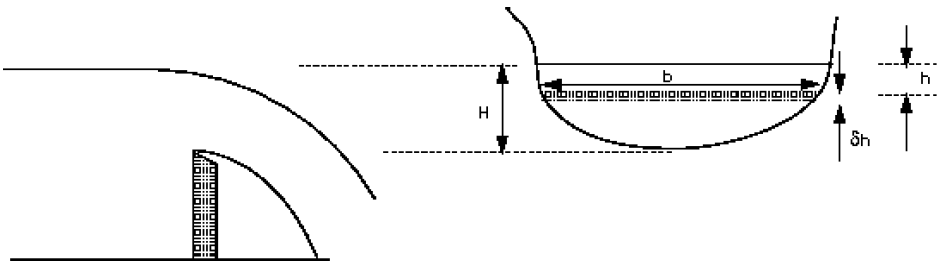
\text{velocity through the strip, }u=\sqrt{2gh}

\text{discharge through the strip, }\delta Q=Au=b\;\delta h\sqrt{2gh}

integrating from the free surface, $h=0$ , to the weir crest, $h=H$ gives the expression for the total theoretical discharge

Q_{\text{theoretical}}=\sqrt{2g}\int_{0}^{H}bh^{1/2}\;dh

This will be different for every differently shaped weir or notch. To make further use of this equation we need an expression relating the width of flow across the weir to the depth below the free surface.

4.17.3 Rectangular Weir

For a rectangular weir the width does not change with depth so there is no relationship between b and depth h. We have the equation,

b=\text{constant }=B

Substituting this into the general weir equation gives

	$\displaystyle Q_{\text{theoretical}}$	$\displaystyle=B\sqrt{2g}\int_{0}^{H}h^{1/2}\;dh$
		$\displaystyle=\frac{2}{3}B\sqrt{2g}H^{3/2}$

To calculate the actual discharge we introduce a coefficient of discharge, $C_{d}$ , which accounts for losses at the edges of the weir and contractions in the area of flow, giving

Q_{\text{actual}}=C_{d}\frac{2}{3}B\sqrt{2g}H^{3/2}

4.17.4 ’V’ Notch Weir

For the ”V” notch weir the relationship between width and depth is dependent on the angle of the ”V”.

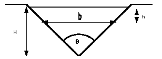
If the angle of the ”V” is $\theta$ then the width, $b$ , a depth $h$ from the free surface is

b=2(H-h)\tan\left(\frac{\theta}{2}\right)

So the discharge is

	$\displaystyle Q_{\text{theoretical}}$	$\displaystyle=2\sqrt{2g}\tan\left(\frac{\theta}{2}\right)\int_{0}^{H}(H-h)h^{1% /2}\;dh$
		$\displaystyle=2\sqrt{2g}\tan\left(\frac{\theta}{2}\right)\left[\frac{2}{5}Hh^{% 3/2}-\frac{2}{5}h^{5/2}\right]^{H}_{0}$
		$\displaystyle=\frac{8}{15}\sqrt{2g}\tan\left(\frac{\theta}{2}\right)H^{5/2}$

And again, the actual discharge is obtained by introducing a coefficient of discharge

Q_{\text{actual}}=C_{d}\frac{8}{15}\sqrt{2g}\tan\left(\frac{\theta}{2}\right)H% ^{5/2}

4.18 Forces in Moving Fluids

4.18.1 The Momentum Equation And Its Applications

We have all seen moving fluids exerting forces. The lift force on an aircraft is exerted by the air moving over the wing. A jet of water from a hose exerts a force on whatever it hits. In fluid mechanics the analysis of motion is performed in the same way as in solid mechanics - by use of Newton’s laws of motion. Account is also taken for the special properties of fluids when in motion.

The momentum equation is a statement of Newton’s Second Law and relates the sum of the forces acting on an element of fluid to its acceleration or rate of change of momentum. You will probably recognise the equation $F=ma$ which is used in the analysis of solid mechanics to relate applied force to acceleration. In fluid mechanics it is not clear what mass of moving fluid we should use so we use a different form of the equation.

Newton’s 2nd Law can be written:

The Rate of change of momentum of a body is equal to the resultant force acting on the body, and takes place in the direction of the force.

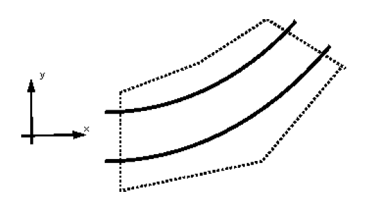
To determine the rate of change of momentum for a fluid we will consider a streamtube as we did for the Bernoulli equation,

We start by assuming that we have steady flow which is non-uniform flowing in a stream tube.

In time $\delta t$ a volume of the fluid moves from the inlet a distance $u\;\delta t$ , so the volume entering the streamtube in the time $\delta t$ is

\text{volume entering the stream tube }=\text{area }\times\text{distance}=A_{1% }u_{1}\delta t

this has mass,

\text{mass entering the stream tube }=\text{density }\times\text{volume}=\rho_% {1}A_{1}u_{1}\delta t

and momentum

\text{momentum of fluid entering the stream tube }=\text{mass }\times\text{% velocity}=\rho_{1}A_{1}u_{1}\delta tu_{1}

Similarly, at the exit, we can obtain an expression for the momentum leaving the steamtube:

\text{momentum of fluid {leaving} the stream tube }=\rho_{2}A_{2}u_{2}\delta tu% _{2}

We can now calculate the force exerted by the fluid using Newton’s 2nd Law. The force is equal to the rate of change of momentum. So

	Force	$\displaystyle=\text{rate of change of momentum}$
	$\displaystyle F$	$\displaystyle=\frac{(\rho_{2}A_{2}u_{2}\delta tu_{2}-\rho_{1}A_{1}u_{1}\delta tu% _{1})}{\delta t}$

We know from continuity that $Q=A_{1}u_{1}=A_{2}u_{u}$ , and if we have a fluid of constant density, i.e. $\rho_{1}=\rho_{2}=\rho$ , then we can write

F=\rho Q(u_{2}-u_{1})

For an alternative derivation of the same expression, as we know from conservation of mass in a stream tube that

\text{mass into face 1}=\text{mass out of face 2}

we can write

\text{rate of change of mass}=\dot{m}=\frac{dm}{dt}=\rho_{1}A_{1}u_{1}=\rho_{2% }A_{2}u_{2}

The rate at which momentum enters face 1 is

\rho_{1}A_{1}u_{1}u_{1}=\dot{m}u_{1}

The rate at which momentum leaves face 2 is

\rho_{2}A_{2}u_{2}u_{2}=\dot{m}u_{2}

Thus the rate at which momentum changes across the stream tube is

\rho_{2}A_{2}u_{2}u_{2}-\rho_{1}A_{1}u_{1}u_{1}=\dot{m}u_{2}-\dot{m}u_{1}

i.e.

	Force	$\displaystyle=\text{rate of change of momentum}$
	$\displaystyle F$	$\displaystyle=\dot{m}(u_{2}-u_{1})$
	$\displaystyle F=\rho Q(u_{2}-u_{1})$

This force is acting in the direction of the flow of the fluid.

This analysis assumed that the inlet and outlet velocities were in the same direction - i.e. a one dimensional system. What happens when this is not the case?

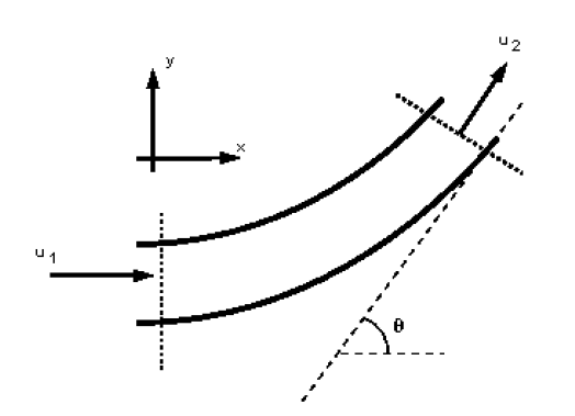
Consider the two dimensional system in the figure below:

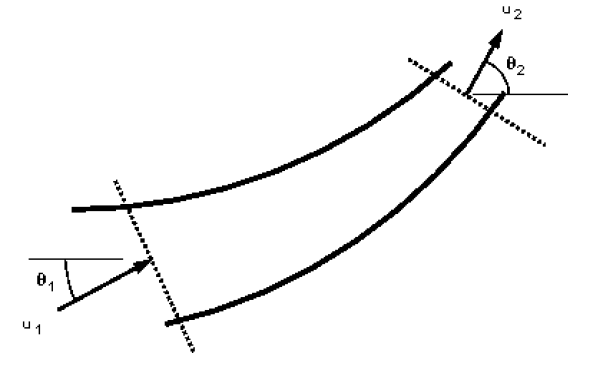
At the inlet the velocity vector, $u_{1}$ , makes an angle, $\theta_{1}$ , with the $x$ -axis, while at the outlet $u_{2}$ makes an angle $\theta_{2}$ . In this case we consider the forces by resolving in the directions of the co-ordinate axes.

The force in the $x$ -direction

	$\displaystyle F_{x}$	$\displaystyle=\text{rate of change of momentum in x-direction}$
		$\displaystyle=\text{rate of change of mass }\times\text{change in velocity in % x-direction}$
		$\displaystyle=\dot{m}\left(u_{2}\cos\theta_{2}-u_{1}\cos\theta_{1}\right)$
		$\displaystyle=\dot{m}\left({u_{2}}_{x}-{u_{1}}_{x}\right)$
		$\displaystyle=\rho Q\left(u_{2}\cos\theta_{2}-u_{1}\cos\theta_{1}\right)$
		$\displaystyle=\rho Q\left({u_{2}}_{x}-{u_{1}}_{x}\right)$

And the force in the $y$ -direction

	$\displaystyle F_{x}$	$\displaystyle=\dot{m}\left(u_{2}\sin\theta_{2}-u_{1}\sin\theta_{1}\right)$
		$\displaystyle=\dot{m}\left({u_{2}}_{y}-{u_{1}}_{y}\right)$
		$\displaystyle=\rho Q\left(u_{2}\sin\theta_{2}-u_{1}\sin\theta_{1}\right)$
		$\displaystyle=\rho Q\left({u_{2}}_{y}-{u_{1}}_{y}\right)$

We then find the resultant force by combining these vectorially:

F_{\text{resultant}}=\sqrt{F_{x}^{2}+F_{y}^{2}}

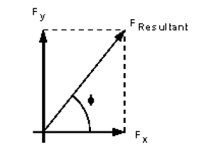
And the angle which this force acts at is given by

\phi=\tan^{-}1\left(\frac{F_{y}}{F_{x}}\right)

For a three-dimensional ( $x$ , $y$ , $z$ ) system we then have an extra force to calculate and resolve in the $z$ -direction. This is considered in exactly the same way.

In summary we can say:

	The total force excerted on the fluid	$\displaystyle=\text{rate of change of momentum through the control volume}$
	$\displaystyle F$	$\displaystyle=\dot{m}\left(u_{\text{out}}-u_{\text{in}}\right)$
		$\displaystyle=\rho Q\left(u_{\text{out}}-u_{\text{in}}\right)$

Remember that we are working with vectors so F is in the direction of the velocity. This force is made up of three components:

•

$F_{R}=$ Force exerted on the fluid by any solid body touching the control volume
•

$F_{B}=$ Force exerted on the fluid body (e.g. gravity)
•

$F_{p}=$ Force exerted on the fluid by fluid pressure outside the control volume

So we say that the total force, $F_{T}$ , is given by the sum of these forces:

F_{T}=F_{R}+F_{B}+F_{p}

The force exerted by the fluid on the solid body touching the control volume is opposite to $F_{R}$ . So the reaction force, $R$ , is given by

R=-F_{R}

4.19 Application of the Momentum Equation

We will consider the following examples:

1.

Force due to the flow of fluid round a pipe bend.
2.

Force on a nozzle at the outlet of a pipe.
3.

Impact of a jet on a plane surface.
4.

Force due to flow round a curved vane.

4.19.1 The force due the flow around a pipe bend

Consider a pipe bend with a constant cross section lying in the horizontal plane and turning through an angle of $\theta^{o}$ .

Why do we want to know the forces here? Because the fluid changes direction, a force (very large in the case of water supply pipes,) will act in the bend. If the bend is not fixed it will move and eventually break at the joints. We need to know how much force a support (thrust block) must withstand.

Step in Analysis:

1.

Draw a control volume
2.

Decide on co-ordinate axis system
3.

Calculate the total force
4.

Calculate the pressure force
5.

Calculate the body force
6.

Calculate the resultant force

1. Control Volume

The control volume is draw in the above figure, with faces at the inlet and outlet of the bend and encompassing the pipe walls.

2. Co-ordinate axis system

It is convenient to choose the co-ordinate axis so that one is pointing in the direction of the inlet velocity. In the above figure the x-axis points in the direction of the inlet velocity.

3. Calculate the total force

In the $x$ -direction:

F_{Tx}=\rho Q\left(u_{2x}-u_{1x}\right)

u_{1x}=u_{1}

u_{2x}=u_{2}\cos\theta

F_{Tx}=\rho Q\left(u_{2}\cos\theta-u_{1}\right)

In the $y$ -direction:

F_{Ty}=\rho Q\left(u_{2y}-u_{1y}\right)

u_{1y}=u_{1}\sin 0=0

u_{2y}=u_{2}\sin\theta

F_{Ty}=\rho Qu_{2}\sin\theta

4. Calculate the pressure force

F_{P}=\text{pressure force at 1}-\text{pressure force at 2}

	$\displaystyle F_{P_{x}}$	$\displaystyle=p_{1}A_{1}\cos 0-p_{2}A_{2}\cos\theta=p_{1}A_{1}-p_{2}A_{2}\cos\theta$
	$\displaystyle F_{P_{y}}$	$\displaystyle=p_{1}A_{1}\sin 0-p_{2}A_{2}\sin\theta=-p_{2}A_{2}\sin\theta$

5. Calculate the body force

There are no body forces in the $x$ or $y$ directions. The only body force is that exerted by gravity (which acts into the paper in this example - a direction we do not need to consider).

6. Calculate the resultant force

	$\displaystyle F_{Tx}$	$\displaystyle=F_{Rx}+F_{Px}+F_{Bx}$
	$\displaystyle F_{Ty}$	$\displaystyle=F_{Ry}+F_{Py}+F_{By}$

	$\displaystyle F_{Rx}$	$\displaystyle=F_{Tx}-F_{Px}-0=\rho Q\left(u_{2}\cos\theta-u_{1}\right)-p_{1}A_% {1}+p_{2}A_{2}\cos\theta$
	$\displaystyle F_{Ry}$	$\displaystyle=F_{Ty}-F_{Py}-0=\rho Qu_{2}\sin\theta+p_{2}A_{2}\sin\theta$

And the resultant force on the fluid is given by

F_{R}=\sqrt{F_{Rx}^{2}-F_{Ry}^{2}}

And the direction of application is

\phi=\tan^{-1}\left(\frac{F_{Ry}}{F_{Rx}}\right)

the force on the bend is the same magnitude but in the opposite direction

R=-F_{R}

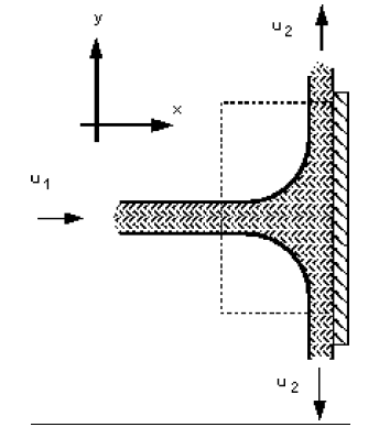
4.19.2 Force on a pipe nozzle

Force on the nozzle at the outlet of a pipe. Because the fluid is contracted at the nozzle forces are induced in the nozzle. Anything holding the nozzle (e.g. a fireman) must be strong enough to withstand these forces.

The analysis takes the same procedure as above:

1.

Draw a control volume
2.

Decide on co-ordinate axis system
3.

Calculate the total force
4.

Calculate the pressure force
5.

Calculate the body force
6.

Calculate the resultant force

1. & 2. Control volume and Co-ordinate axis are shown in the figure below.

Notice how this is a one dimensional system which greatly simplifies matters.

3. Calculate the total force

F_{T}=F_{Tx}=\rho Q\left(u_{2}-u_{1}\right)

By continuity, $Q=A_{1}u_{1}=A_{2}u_{2}$ , so

F_{Tx}=\rho Q^{2}\left(\frac{1}{A^{2}}-\frac{1}{A_{1}}\right)

4. Calculate the pressure force

F_{P}=F_{Px}=\text{pressure force at 1}-\text{pressure force at 2}

We use the Bernoulli equation to calculate the pressure

\frac{p_{1}}{\rho g}+\frac{u_{1}}{2g}+z_{1}=\frac{p_{2}}{\rho g}+\frac{u_{2}}{% 2g}+z_{2}+h_{f}

If friction losses are neglected, $h_{f}=0$

As the nozzle is horizontal, $z_{1}=z_{2}$

and as the pressure outside is atmospheric, we can say $p_{2}=0$ , and $p_{1}$ we can calculate as gauge pressure. Together with continuity these give:

p_{1}=\frac{\rho Q^{2}}{2}\left(\frac{1}{A_{2}^{2}}-\frac{1}{A_{1}^{2}}\right)

5. Calculate the body force

The only body force is the weight due to gravity in the y-direction - but we need not consider this as the only forces we are considering are in the x-direction.

6. Calculate the resultant force

	$\displaystyle F_{Tx}$	$\displaystyle=F_{Rx}+F_{Px}+F_{Bx}$
	$\displaystyle F_{Rx}$	$\displaystyle=F_{Tx}-F_{Py}-0$

F_{Tx}=\rho Q^{2}\left(\frac{1}{A_{2}}-\frac{1}{A_{1}}\right)-\frac{\rho Q^{2}% }{2}\left(\frac{1}{A_{2}^{2}}-\frac{1}{A_{1}^{2}}\right)

So the fireman must be able to resist the force of

R=-F_{Tx}

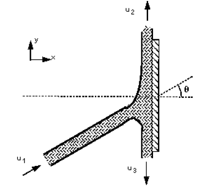
4.19.3 Impact of a Jet on a Plane

We will first consider a jet hitting a flat plate (a plane) at an angle of $90^{\circ}$ , as shown in the figure below.

We want to find the reaction force of the plate i.e. the force the plate will have to apply to stay in the same position.

The analysis take the same procedure as above:

1.

Draw a control volume
2.

Decide on co-ordinate axis system
3.

Calculate the total force
4.

Calculate the pressure force
5.

Calculate the body force
6.

Calculate the resultant force

1. & 2. Control volume and Co-ordinate axis are shown in the figure below.

3. Calculate the total force

	$\displaystyle F_{Tx}$	$\displaystyle=\rho Q\left(u_{2x}-u_{1x}\right)$
		$\displaystyle=-\rho Qu_{1x}$

As the system is symmetrical the forces in the y-direction cancel i.e.

F_{Ty}=0

4. Calculate the pressure force

The pressure force is zero as the pressure at both the inlet and the outlets to the control volume are atmospheric.

5. Calculate the body force

As the control volume is small we can ignore the body force due to the weight of gravity.

6. Calculate the resultant force

	$\displaystyle F_{Tx}$	$\displaystyle=F_{Rx}+F_{Px}+F_{Bx}$
	$\displaystyle F_{Rx}$	$\displaystyle=F_{Tx}-0-0$
		$\displaystyle=-\rho Qu_{1x}$

This force is exerted on the fluid.

The force on the plane is the same magnitude but in the opposite direction

R=-F_{Rx}

4.19.4 Force on a curved vane

This case is similar to that of a pipe, but the analysis is simpler because the pressures are equal - i.e. atmospheric pressure, and both the cross-section and velocities (in the direction of flow) remain constant. The jet, vane and co-ordinate direction are arranged as in the figure below.

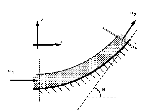
1. & 2. Control volume and Co-ordinate axis are shown in the figure above.

3. Calculate the total force in the x direction

F_{Tx}=\rho Q\left(u_{2}-u_{1}\cos\theta\right)

but $u_{1}=u_{2}=\frac{Q}{A}$ , so

F_{Tx}=-\rho\frac{Q^{2}}{A}\left(1-\cos\theta\right)

and in the y-direction

	$\displaystyle F_{Ty}$	$\displaystyle=\rho Q\left(u_{2}\sin\theta-0\right)$
		$\displaystyle=\rho\frac{Q^{2}}{A}$

4. Calculate the pressure force.

Again, the pressure force is zero as the pressure at both the inlet and the outlets to the control volume are atmospheric.

5. Calculate the body force No body forces in the x-direction, $F_{Bx}=0$ . In the y-direction the body force acting is the weight of the fluid. If V is the volume of the fluid on he vane then,

F_{Bx}=\rho gV

(This is often small is the jet volume is small and sometimes ignored in analysis.)

6. Calculate the resultant force

	$\displaystyle F_{Tx}$	$\displaystyle=F_{Rx}+F_{Px}+F_{Bx}$
	$\displaystyle F_{Rx}$	$\displaystyle=F_{Tx}$
	$\displaystyle F_{Ty}$	$\displaystyle=F_{Ry}+F_{Py}+F_{By}$
	$\displaystyle F_{Ry}$	$\displaystyle=F_{Ty}$

And the resultant force on the fluid is given by

F_{R}=\sqrt{F_{Rx}^{2}-F_{Ry}^{2}}

And the direction of application is

\phi=\tan\left(\frac{F_{Ry}}{F_{Rx}}\right)

exerted on the fluid.

The force on the vane is the same magnitude but in the opposite direction

R=-F_{R}

4.19.5 Pelton wheel blade

The above analysis of impact of jets on vanes can be extended and applied to analysis of turbine blades. One particularly clear demonstration of this is with the blade of a turbine called the pelton wheel. The arrangement of a pelton wheel is shown in the figure below. A narrow jet (usually of water) is fired at blades which stick out around the periphery of a large metal disk. The shape of each of these blade is such that as the jet hits the blade it splits in two (see figure below) with half the water diverted to one side and the other to the other. This splitting of the jet is beneficial to the turbine mounting - it causes equal and opposite forces (hence a sum of zero) on the bearings.

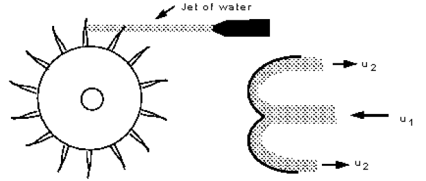
A closer view of the blade and control volume used for analysis can be seen in the figure below.

Analysis again take the following steps:

1.

Draw a control volume
2.

Decide on co-ordinate axis system
3.

Calculate the total force
4.

Calculate the pressure force
5.

Calculate the body force
6.

Calculate the resultant force

1 & 2 Control volume and Co-ordinate axis are shown in the figure below.

3 Calculate the total force in the x direction

F_{Tx}=\rho\left(\frac{Q}{2}u_{2x}+\frac{Q}{2}u_{2x}-Qu_{1x}\right)

	$\displaystyle u_{1x}$	$\displaystyle=-u_{1}$
	$\displaystyle u_{2x}$	$\displaystyle=u_{2}\cos\theta$

F_{Tx}=\rho Q\left(u_{2}\cos\theta+u_{1}\right)

and in the y-direction it is symmetrical, so

F_{Ty}=0

4 Calculate the pressure force.

The pressure force is zero as the pressure at both the inlet and the outlets to the control volume are atmospheric.

5 Calculate the body force

We are only considering the horizontal plane in which there are no body forces.

6 Calculate the resultant force

	$\displaystyle F_{Tx}$	$\displaystyle=F_{Rx}+F_{Px}+F_{Bx}$
	$\displaystyle F_{Rx}$	$\displaystyle=F_{Tx}-0-0$
		$\displaystyle=\rho Q\left(u_{2}\cos\theta+u_{1}\right)$

exerted on the fluid.

The force on the blade is the same magnitude but in the opposite direction

R=-F_{Rx}

So the blade moved in the x-direction.

In a real situation the blade is moving. The analysis can be extended to include this by including the amount of momentum entering the control volume over the time the blade remains there. This will be covered in the level 2 module next year.

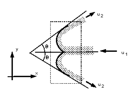
4.19.6 Force due to a jet hitting an inclined plane

We have seen above the forces involved when a jet hits a plane at right angles. If the plane is tilted to an angle the analysis becomes a little more involved. This is demonstrated below.

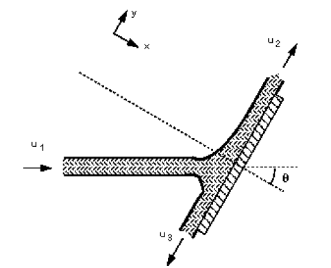
(Note that for simplicity gravity and friction will be neglected from this analysis.)

We want to find the reaction force normal to the plate so we choose the axis system as above so that is normal to the plane. The diagram may be rotated to align it with these axes and help comprehension, as shown below

We do not know the velocities of flow in each direction. To find these we can apply Bernoulli equation

\frac{p_{1}}{\rho g}+\frac{u_{1}^{2}}{2g}+z_{1}=\frac{p_{2}}{\rho g}+\frac{u_{% 2}^{2}}{2g}+z_{2}=\frac{p_{3}}{\rho g}+\frac{u_{3}^{2}}{2g}+z_{3}

The height differences are negligible i.e. $z_{1}=z_{2}=z_{3}$ and the pressures are all atmospheric $p_{1}=p_{2}=p_{3}$ . So $u_{1}=u_{2}=u_{3}=u$

By continuity

Q_{1}=Q_{2}+Q_{3}

u_{1}A_{1}=u_{2}A_{2}+u_{3}A_{3}

so

A_{1}=A_{2}+A_{3}

Q_{1}=A_{1}u

Q_{2}=A_{2}u

Q_{3}=(A_{1}-A_{2})u

Using this we can calculate the forces in the same way as before.

1.

Draw a control volume
2.

Decide on co-ordinate axis system
3.

Calculate the total force
4.

Calculate the pressure force
5.

Calculate the body force
6.

Calculate the resultant force

3. Calculate the total force in the x-direction.

Remember that the co-ordinate system is normal to the plate.

F_{Tx}=\rho\left(\left(Q_{2}u_{2x}+Q_{3}u_{3x}\right)-Q_{1}u_{1x}\right)

but $u_{2x}=u_{3x}=0$ as the jets are parallel to the plate with no component in the x-direction. $u_{1x}=u_{1}\cos\theta$ , so

F_{Tx}=-\rho Q_{1}u_{1}\cos\theta

4. Calculate the pressure force

All zero as the pressure is everywhere atmospheric.

5. Calculate the body force

As the control volume is small, hence the weight of fluid is small, we can ignore the body forces.

6. Calculate the resultant force

	$\displaystyle F_{Tx}$	$\displaystyle=F_{Rx}+F_{Px}+F_{Bx}$
	$\displaystyle F_{Rx}$	$\displaystyle=F_{Tx}-0-0$
		$\displaystyle=-\rho Q_{1}u_{1}\cos\theta$

exerted on the fluid.

The force on the plate is the same magnitude but in the opposite direction

	$\displaystyle R$	$\displaystyle=-F_{Rx}$
		$\displaystyle=\rho Q_{1}u_{1}\cos\theta$

We can find out how much discharge goes along in each direction on the plate. Along the plate, in the y-direction, the total force must be zero, $F_{Ty}=0$ .

Also in the y-direction: $u_{1y}=u_{1}\sin\theta$ , $u_{2y}=u_{2}$ , $u_{3y}=-u_{3}$ , so

	$\displaystyle F_{Ty}$	$\displaystyle=\rho\left(\left(Q_{2}u_{2y}+Q_{3}u_{3y}\right)-Q_{1}u{1y}\right)$
	$\displaystyle F_{Ty}$	$\displaystyle=\rho\left(Q_{2}u_{2}+Q_{3}u_{3}-Q_{1}u_{1}\sin\theta\right)$

As forces parallel to the plate are zero,

0=\rho A_{2}u_{2}^{2}-\rho A_{3}u_{3}^{2}-\rho A_{1}u_{1}^{2}\sin\theta

From above $u_{1}=u_{2}=u_{3}$

0=A_{2}-A_{3}-A_{1}\sin\theta

and from above we have $A_{1}=A_{2}+A_{3}$ so

	$\displaystyle 0$	$\displaystyle=A_{2}-A_{3}-\left(A_{2}+A_{3}\right)\sin\theta$
		$\displaystyle=A_{2}\left(1-\sin\theta\right)-A_{3}\left(1+\sin\theta\right)$
	$\displaystyle A_{2}$	$\displaystyle=A_{3}\left(\frac{1+\sin\theta}{1-\sin\theta}\right)$

as $u_{2}=u_{3}=u$

Q_{2}=Q_{3}\left(\frac{1+\sin\theta}{1-\sin\theta}\right)

	$\displaystyle Q_{1}$	$\displaystyle=Q_{3}\left(\frac{1+\sin\theta}{1-\sin\theta}\right)+Q_{3}$
		$\displaystyle=Q_{3}\left(1+\frac{1+\sin\theta}{1-\sin\theta}\right)$

So we know the discharge in each direction