Laminar and Turbulent Flow
The flow of real fluids exhibits viscous effect, that is they
tend to "stick" to solid surfaces and have stresses
within their body.
You might remember from earlier in the course Newtons law of viscosity:

This tells us that the shear stress, t, in a fluid is proportional to the velocity gradient - the rate of change of velocity across the fluid path. For a "Newtonian" fluid we can write:

where the constant of proportionality, m,
is known as the coefficient of viscosity (or simply viscosity).
We saw that for some fluids - sometimes known as exotic fluids
- the value of m changes with
stress or velocity gradient. We shall only deal with Newtonian
fluids.
In his lecture we shall look at how the forces due to momentum
changes on the fluid and viscous forces compare and what changes
take place.
2. Laminar and turbulent flow
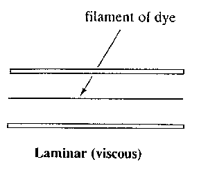
If we were to take a pipe of free flowing water and inject a dye
into the middle of the stream, what would we expect to happen?
This
this
or this
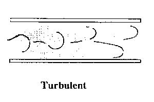
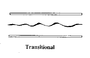
Actually both would happen - but for different flow rates. The
top occurs when the fluid is flowing fast and the lower when it
is flowing slowly.
The top situation is known as turbulent flow and the lower as laminar flow.
In laminar flow the motion of the particles of fluid is very orderly
with all particles moving in straight lines parallel to the pipe
walls.
But what is fast or slow? And at what speed does the flow pattern
change? And why might we want to know this?
The phenomenon was first investigated in the 1880s by Osbourne
Reynolds in an experiment which has become a classic in fluid
mechanics.
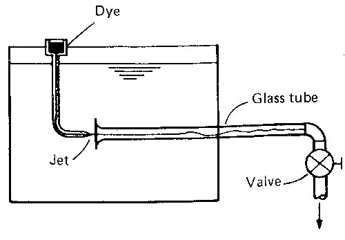
He used a tank arranged as above with a pipe taking water from the centre into which he injected a dye through a needle. After many experiments he saw that this expression

where r = density, u = mean velocity, d = diameter and m = viscosity
would help predict the change in flow type. If the value is less
than about 2000 then flow is laminar, if greater than 4000 then
turbulent and in between these then in the transition zone.
This value is known as the Reynolds number, Re:

Laminar flow: Re < 2000
Transitional flow: 2000 < Re < 4000
Turbulent flow: Re > 4000
What are the units of this Reynolds number? We can fill in the
equation with SI units:
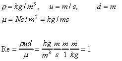
i.e. it has no units. A quantity that has no units
is known as a non-dimensional (or dimensionless) quantity.
Thus the Reynolds number, Re, is a non-dimensional number.
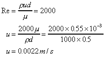
We can go through an example to discover at what velocity the flow in a pipe stops being laminar.
If the pipe and the fluid have the following properties:
water density r = 1000 kg/m3
pipe diameter d = 0.5m
(dynamic) viscosity, m = 0.55x10³
Ns/m2
We want to know the maximum velocity when the Re is 2000.
If this were a pipe in a house central heating system, where the
pipe diameter is typically 0.015m, the limiting velocity for laminar
flow would be, 0.0733 m/s.
Both of these are very slow. In practice it very rarely occurs
in a piped water system - the velocities of flow are much greater.
Laminar flow does occur in situations with fluids of greater viscosity
- e.g. in bearing with oil as the lubricant.
At small values of Re above 2000 the flow exhibits small instabilities.
At values of about 4000 we can say that the flow is truly turbulent.
Over the past 100 years since this experiment, numerous more experiments
have shown this phenomenon of limits of Re for many different
Newtonian fluids - including gasses.
What does this abstract number mean?
We can say that the number has a physical meaning, by doing so it helps to understand some of the reasons for the changes from laminar to turbulent flow.
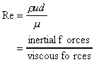
It can be interpreted that when the inertial forces dominate over
the viscous forces (when the fluid is flowing faster and Re is
larger) then the flow is turbulent. When the viscous forces are
dominant (slow flow, low Re) they are sufficient enough to keep
all the fluid particles in line, then the flow is laminar.
In summary:
Laminar flow
- Re < 2000
- 'low' velocity
- Dye does not mix with water
- Fluid particles move in straight lines
- Simple mathematical analysis possible
- Rare in practice in water systems.
Transitional flow
- 2000 > Re < 4000
- 'medium' velocity
- Dye stream wavers in water - mixes slightly.
Turbulent flow
- Re > 4000
- 'high' velocity
- Dye mixes rapidly and completely
- Particle paths completely irregular
- Average motion is in the direction of the flow
- Cannot be seen by the naked eye
- Changes/fluctuations are very difficult to detect. Must use laser.
- Mathematical analysis very difficult - so experimental measures are used
- Most common type of flow.
3. Pressure loss due to friction in a pipeline.
Up to this point on the course we have considered ideal fluids where there have been no losses due to friction or any other factors. In reality, because fluids are viscous, energy is lost by flowing fluids due to friction which must be taken into account. The effect of the friction shows itself as a pressure (or head) loss.
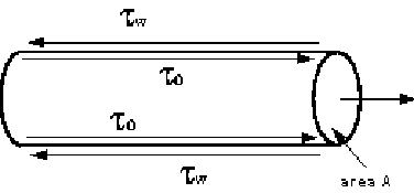
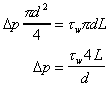
In a pipe with a real fluid flowing, at the wall there is a shearing stress retarding the flow, as shown below.
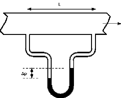
If a manometer is attached as the pressure (head) difference due to the energy lost by the fluid overcoming the shear stress can be easily seen.
The pressure at 1 (upstream) is higher than the pressure at 2.
We can do some analysis to express this loss in pressure in terms of the forces acting on the fluid.
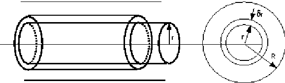
Consider a cylindrical element of incompressible fluid flowing in the pipe, as shown
The pressure at the upstream end is p, and at the downstream end the pressure has fallen by Dp to (p-Dp).
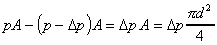
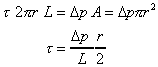
The driving force due to pressure (F = Pressure x Area) can then be written
driving force = Pressure force at 1 - pressure force at 2
The retarding force is that due to the shear stress by the walls
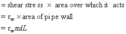
As the flow is in equilibrium,
driving force = retarding force
Giving an expression for pressure loss in a pipe in terms of the pipe diameter and the shear stress at the wall on the pipe.
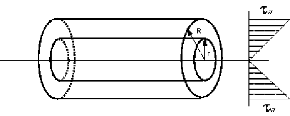
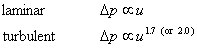
The shear stress will vary with velocity of flow and hence with Re. Many experiments have been done with various fluids measuring the pressure loss at various Reynolds numbers. These results plotted to show a graph of the relationship between pressure loss and Re look similar to the figure below:
This graph shows that the relationship between pressure loss and Re can be expressed as
As these are empirical relationships, they help in determining the pressure loss but not in finding the magnitude of the shear stress at the wall tw on a particular fluid. If we knew tw we could then use it to give a general equation to predict the pressure loss.
4. Pressure loss during laminar flow in a pipe
In general the shear stress tw. is almost impossible to measure. But for laminar flow it is possible to calculate a theoretical value for a given velocity, fluid and pipe dimension.
In laminar flow the paths of individual particles of fluid do not cross, so the flow may be considered as a series of concentric cylinders sliding over each other - rather like the cylinders of a collapsible pocket telescope.
As before, consider a cylinder of fluid, length L, radius r, flowing steadily in the centre of a pipe.
We are in equilibrium, so the shearing forces on the cylinder equal the pressure forces.
By Newtons law of viscosity we have  ,
where y is the distance from the wall. As we are measuring from
the pipe centre then we change the sign and replace y with r distance
from the centre, giving
,
where y is the distance from the wall. As we are measuring from
the pipe centre then we change the sign and replace y with r distance
from the centre, giving

Which can be combined with the equation above to give

In an integral form this gives an expression for velocity,
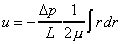
Integrating gives the value of velocity at a point distance r from the centre
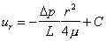
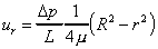
At r = 0, (the centre of the pipe), u = umax, at r = R (the pipe wall) u = 0, giving

so, an expression for velocity at a point r from the pipe centre when the flow is laminar is
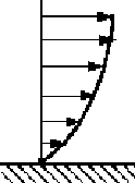
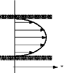
Note how this is a parabolic profile (of the form y = ax2 + b ) so the velocity profile in the pipe looks similar to the figure below
What is the discharge in the pipe?
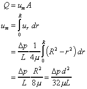
So the discharge can be written
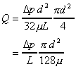
This is the Hagen-Poiseuille equation for laminar flow in a pipe.
It expresses the discharge Q in terms of the pressure gradient
( ), diameter of the pipe and the viscosity
of the fluid.
), diameter of the pipe and the viscosity
of the fluid.
We are interested in the pressure loss (head loss) and want to
relate this to the velocity of the flow. Writing pressure loss
in terms of head loss hf, i.e. p = rghf

This shows that pressure loss is directly proportional to the velocity when flow is laminar.
It has been validated many time by experiment.
It justifies two assumptions:
- fluid does not slip past a solid boundary
- Newtons hypothesis.