E3 Questions on Gradually varied flow - including integration of the backwater curve.
-
E3.1
A Rectangular channel is 3.0m wide, has a 0.01 slope, discharge of , and n=0.011. Find and . If the actual depth of flow is 1.7m, what type of profile exists?
(Answer: = 0.4m, = 0.683m, S1 Curve)We need to solve Manning’s equation for for a rectangular channel.
Figure 23: A rectangular channel section For a rectangular channel, we have:
and
so
The Manning’s equation Eq-2 is thus:
This equation must be solved for by a suitable numerical solution (e.g. trial and error or secant method).
This gives for , , and :
At critical depth , and also , so we can use equation Eq-20
For a rectangular channel, this simplifies (using ) to
This can be formulated to be solved explicitly for , eqn Eq-22:
To give
As then the flow is super-critical.
We can calculate the Froude number of normal depth (eqn Eq-16) to confirm this:
As this confirms that uniform flow is super-critical.
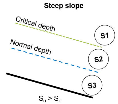
So we have a steep channel, and all surface profiles will be "S" curves.
Figure 24 shows the relative positions of the critical and normal depth lines for a steep slope.
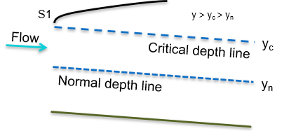
Figure 24: Critical and normal depth lines for a steep slope If at a position in the channel, the depth is , as this is above the critical depth then the profile is in region 1. The surface profile will be an profile. This takes the form as shown in figure 25
Figure 25: The profile -
E3.2
A rectangular channel with a bottom width of and a bottom slope of has a discharge of . In a gradually varied flow in this channel, the depth at a certain location is found to be assuming , determining the type of GVF profile, the critical depth, and the normal depth.
(Answer: M2, , )Following example E3.1, the Manning’s equation Eq-2 is:
This equation must be solved for by a suitable numerical solution (e.g. trial and error or secant method).
This gives for , , and :
At critical depth , and also , so we can use equation Eq-14 equated to 1
For a rectangular channel, this simplifies (using ) to
This can be formulated to be solved explicitly for (eqn Eq-22):
To give
As then the flow is sub-critical.
We can calculate the Froude number of normal depth to confirm this:
As this confirms that uniform flow is sub-critical.
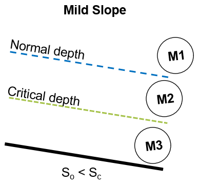
So we have a mild channel, and all surface profiles will be "M" curves.
Figure 26 shows the relative positions of the critical and normal depth lines for a mild slope.
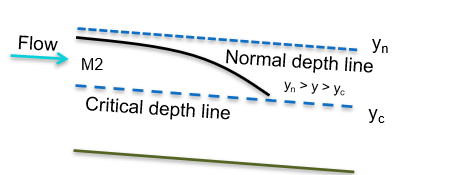
Figure 26: Critical and normal depth lines for a mild slope If at a position in the channel, the depth is , as this is above the critical depth and below the normal depth the profile is in region 2. The surface profile will be an profile. This takes the form as shown in figure 27
Figure 27: The profile -
E3.3
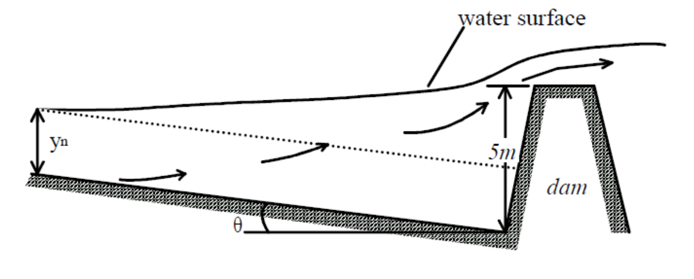
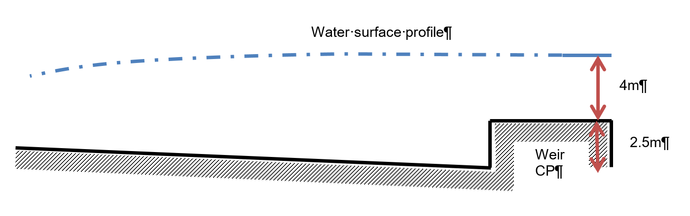
The figure below shows a backwater curve in a long rectangular channel. Determine using a numerical integration method, the profile for the following high flow conditions: , , , and a bed slope of . Take the depth just upstream of the dam as the control point equal to . At what distance is the water level not affected by the dam? perform your integration using a) 2-steps and b) 10-steps
(Answer: .
Using (Euler) 2-step , 10-step .
Using 2-step , 10-step .
Using a forth-order Runge Kutta method gave 2-step , 10-step )Figure 28: The backwater curve for question E3.3 We will integrate using a numerical method that solves to obtain a distance from depth change. There are various methods. We will demonstrate 3 here.
We must solve (integrate) this backwater, or gradually varied flow, equation Eq-42:
Solving for distance, , given a change in depth . So in total differential form, we will solve:
There are options now as to the way the right-hand side is approximated (or discretised). Some options are
For all methods, we calculate and in the same way using the appropriate depth and other channel properties. The equations to use are, for the Froude number, in a rectangular channel (equation Eq-14):
And remembering that is determined from the Manning’s equation (Eq-2), assuming that over the short distance then:
rearranging for and substituting appropriately for a rectangular channel we get from equation Eq-45:
The question asks to find the distance to where the depth is not affected by the dam - this is asking, when does the depth reach normal depth?. So we must first calculate . This is done via a straightforward iteration of the Manning’s equation for a rectangular channel (see previous examples).
In this case using , , and then the solution is, normal depth .
The level just upstream of the dam is , so we need to integrate to find when has dropped to . That is a drop, (so negative), of
We are asked to calculate the distance using a 2-step integration which would give
and also for a 10-step integration which would give
We can now take each of the three discretisation methods and construct an iteration table (e.g. in Excel) for each to calculate the two solutions using the two values.
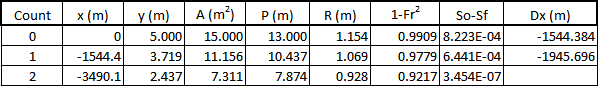
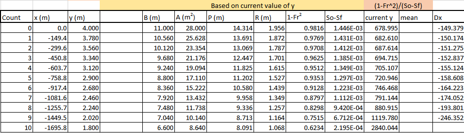
Integration method E3.3i) - First-order Euler
Figure 29 shows the integration table for the 2-step integration and a distance of upstream of the dam to normal depth.
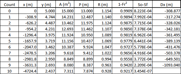
Figure 29: Method E3.3i) Euler integration. 2-steps, Figure 30 shows the integration table for the 10-step integration and a distance of upstream of the dam to normal depth.
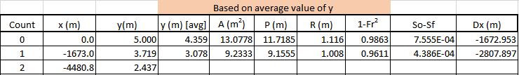
Figure 30: Method E3.3i) Euler integration. 10-steps, Integration method E3.3ii) - Average
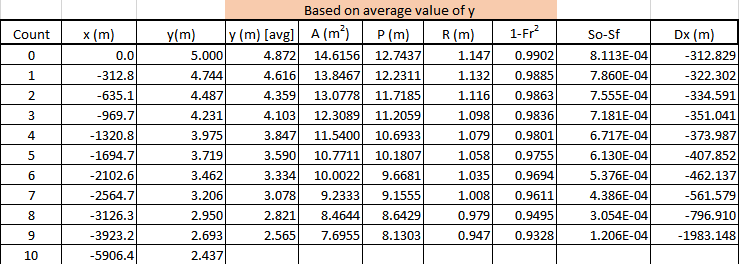
Figure 31 shows the integration table for the 2-step integration and a distance of upstream of the dam to normal depth.
Figure 31: Method E3.3ii) Average integration. 2-steps, Figure 32 shows the integration table for the 10-step integration and a distance of upstream of the dam to normal depth.
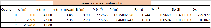
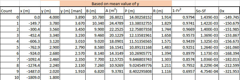
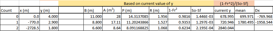
Figure 32: Method E3.3ii) Average integration. 10-steps, Integration method E3.3iii) - Average
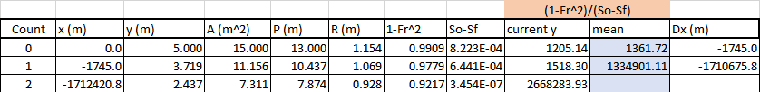
Figure 33 shows the integration table for the 2-step integration and a distance of upstream of the dam to normal depth. This seems incorrect (unlikely), however, let’s have a look a the 10-step solution.
Figure 33: Method E3.3iii) Average integration. 2-steps, Figure 34 shows the integration table for the 10-step integration and a distance of upstream of the dam to normal depth. This again seems incorrect.
Figure 34: Method E3.3iii) Average integration. 10-steps, The reason why this method does not give expected answers is that it fails when depth is equal to . The reason is that would is zero at . In the numerical calculation, it is close to zero, , and gives a very long last . We can say that this method should not be used when the depth of is to be encountered.
A hack that could allow us to use this method would be to perform an Euler step for the last integration step (i.e. avoid the use of ). [We might call this a hybrid method.]. This would give, for the 2-step and for the 10-step .
A fourth-order Runge-Kutta method is usually considered as accurate as practically possible for a numerical method. Using this on the above problem gave for the 2-step , and for the 10-step .
In summary, the solutions are shown in the table 1 below
Table 1: Summary of distances upstream in metres to normal depth from 4 methods -
E3.4
A trapezoidal, concrete-lined, channel has a constant bed slope of , a bed width of , and side slopes of . A control gate increased the depth immediately upstream to . When the discharge is compute the water surface profile upstream and identify the distance when the water depth is . ()
(Answer: Using (Euler) 2-step , 10-step .
Using 2-step , 10-step .
Using mean GVF function: 2-step , 10-step .
Using a forth-order Runge Kutta method gave 2-step , 10-step )This solution follows similarly to that of example question E3.3. We have been given an initial depth of and asked to find the distance upstream to where the depth is .
We should first determine the normal and critical depths. Although these are not directly used in the question, they do inform what solutions is expected and whether the depths rise or fall. The calculations must be done iteratively, as seen in previous examples.
Undertaking the iterative calculation we get and . So flow is sub-critical, and the slope is mild. The depths given for the calculation of the surface are above the normal depth so the surface profile will be a profile. It will slope downwards from 4m toward the target of 1.8m.
The depth fall is a drop, (so negative), of
We are asked to calculate the distance using a 2-step integration which would give
And also for a 10-step integration which would give
Here we demonstrate results from the three integration methods identified in example E3.3 above.
Integration method E3.3i) - First-order Euler
Figure 35 shows the integration table for the 2-step integration and a distance of upstream of the dam to the target depth.
Figure 35: Method E3.3i) Euler integration. 2-steps, Figure 36 shows the integration table for the 10-step integration and a distance of upstream of the dam to the target depth.
Figure 36: Method E3.3i) Euler integration. 10-steps, Integration method E3.3ii) - Average
Figure 37 shows the integration table for the 2-step integration and a distance of upstream of the dam to the target depth.
Figure 37: Method E3.3ii) Average integration. 2-steps, Figure 38 shows the integration table for the 10-step integration and a distance of upstream of the dam to the target depth.
Figure 38: Method E3.3ii) Average integration. 10-steps, Integration method E3.3iii) - Average
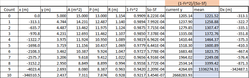
Figure 39 shows the integration table for the 2-step integration and a distance of upstream of the dam to the target depth. This seems incorrect (unlikely), however, let’s have a look a the 10-step solution.
Figure 39: Method E3.3iii) Average integration. 2-steps, Figure 40 shows the integration table for the 10-step integration and a distance of upstream of the dam to the target depth. This again seems incorrect.
Figure 40: Method E3.3iii) Average integration. 10-steps, A fourth-order Runge-Kutta method is usually considered as accurate as practically possible for a numerical method. Using this on the above problem gave for the 2-step , and for the 10-step . A 100-step Runge Kutta give , so the 10-step can probably be considered sufficiently accurate.
In summary, the solutions are shown in the table 1 below
Table 2: Summary of distances upstream in metres to target depth from 4 methods -
E3.5
Using the figure below, determine the profile for the channel conditions using a step length of . , , the bed slope of the rectangular channel is and has a width of . The sill height of the weir is and the water depth over the weir is . Compare results from each method.
Figure 41: The backwater curve for question E3.5 The question is asking to integrate upstream from a depth of at the weir enough distance to understand and compare the flow profile for each method. It suggests an integration step of which should be used for the depth from distance integration. It does not specify that this should be the method so the method integration distance from depth will also be used and the results compared.
We should first understand the flow regime by calculation normal and critical depths and by comparison examine the expected flow profile.
We have a rectangular channel and Manning’s n, so will use the following uniform flow equation:
This equation must be solved for by a suitable numerical solution (e.g. trial and error or secant method).
This gives for , , and :
At critical depth , and also , so we can use the equation Eq-19, written for a rectangular channel
And formulated to solve for critical depth , giving from equation Eq-22
As then uniform flow is sub-critical. The slope of the channel is mild. The depth at the weir is higher that normal depth and moving upstream must fall gradually toward normal depth. This is the region 1 (above normal fro a mild slope), so the profile must be an M1 profile.
The first integration will be the following depth from distance, using and we will use am Euler method i.e. use the conditions at the known point to calculate the derivative. Equation Eq-53
Where the friction slope, , term is, as previously, equation Eq-45:
And the Froude number squared, equation Eq-14
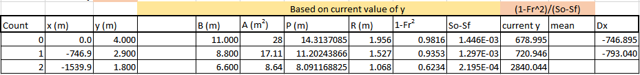
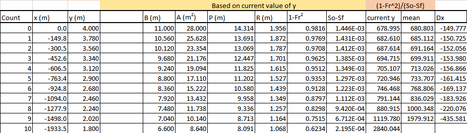
See previous questions for a greater description of the Euler integration methodology. Tabulating the calculation and produces the integration table in figure 42. The integration has been performed for 20 steps and depth has fallen to . Which indicates that normal depth has still not been achieved upstream of the weir.
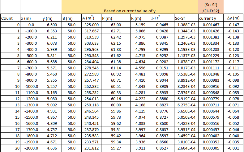
Figure 42: Integration table for fixed As we wish to compare results from a distance from depth integration we should select appropriate parameters. The integration above used 20 steps and reached as depth of . Using these as parameters would give a and 20 steps of integration.
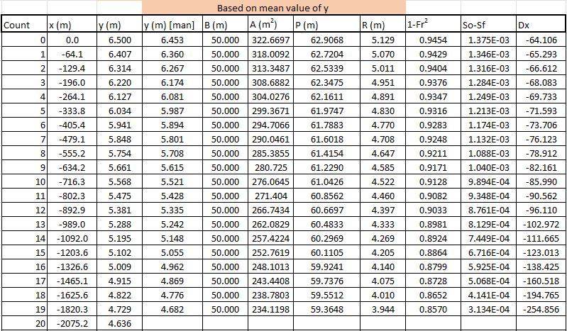
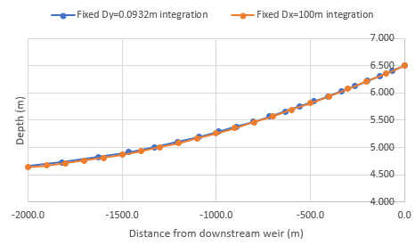
Figure 43: Integration table for fixed and 20 steps Results in an integration table using a derivative approximated at is shown in figure 43. We see from the table that there is a slight difference in the distance to that same depth of . To investigate any further differences by plotting a graph of the two profiles. Such a graph is shown in figure 44. It is clear that the two integrations are very similar - differing by only millimeters along the whole profile length. The shape of the profile is as expected that of an M1 profile.
Figure 44: Integrated Water Profile from the weir upstream for the two integration methods